Highway Safety Benefit-Cost Analysis Guide

Highway Safety Beneﬁt–Cost

Analysis Guide

http://safety.fhwa.dot.gov

FHWA Safety Program

HIGHWAY SAFETY BENEFIT COST ANALYSIS GUIDE

FOREWORD

The purpose of the Highway Safety Benefit-Cost Analysis Guide (this Guide) is to assist

transportation agencies in making consistent and theoretically sound decisions for economically

evaluating and ranking safety countermeasures. Transportation professionals can use the

methods described to analyze both site-specific and systemic safety approaches with single or

multiple countermeasures. This Guide is intended as a user-friendly technical reference which

transportation professionals can use with no prior experience with economic evaluation

techniques. This Guide provides example calculations throughout the document to assist

transportation professionals in understanding benefit-cost analysis (BCA) concepts and applying

them for safety applications.

NOTICE

This document is disseminated under the sponsorship of the U.S. Department of

Transportation in the interest of information exchange. The U.S. Government assumes no

liability for the use of the information contained in this document.

The U.S. Government does not endorse products or manufacturers. Trademarks or

manufacturers’ names appear in this report only because they are considered essential to the

objective of the document.

QUALITY ASSURANCE STATEMENT

The Federal Highway Administration (FHWA) provides high-quality information to serve

Government, industry, and the public in a manner that promotes public understanding.

Standards and policies are used to ensure and maximize the quality, objectivity, utility, and

integrity of its information. FHWA periodically reviews quality issues and adjusts its programs

and processes to ensure continuous quality improvement.

HIGHWAY SAFETY BENEFIT COST ANALYSIS GUIDE

TECHNICAL DOCUMENTATION PAGE

1. Report No.

FHWA-SA-18-001

2. Government Accession

No.

3. Recipient's Catalog No.

4. Title and Subtitle

Highway Safety Benefit-Cost Analysis Guide

5. Report Date

February 2018

6. Performing Organization Code

7.Author(s)

Michael Lawrence, Alan Hachey, Geni Bahar, and Frank Gross

8. Performing Organization Report No.

9. Performing Organization Name and Address

VHB

Venture I

940 Main Campus Drive, Suite 500

Raleigh, NC 27606

10. Work Unit No.

11. Contract or Grant No.

DTFH61-16-D-00005 (VHB)

12. Sponsoring Agency Name and Address

Federal Highway Administration Office of Safety

1200 New Jersey Ave., SE

Washington, DC 20590

13. Type of Report and Period

Final Draft Report, August 2016-

February 2018

14. Sponsoring Agency Code

FHWA

15. Supplementary Notes

The contract manager for this report was Karen Scurry, FHWA. The task was led by Jack Faucett Associates.

16. Abstract

The purpose of the Highway Safety Benefit-Cost Analysis (BCA) Guide is to assist transportation agencies in making

consistent and sound investment decisions. The target audience includes transportation professionals such as traffic

engineers, highway safety engineers, and planners conducting highway safety BCA for projects and programs. This Guide

will help these users to quantify the costs, and direct and indirect safety-related benefits of project alternatives. Direct

safety benefits include the expected change in crash frequency and severity. Indirect benefits include the operational and

environmental benefits that result from a reduction in crashes (e.g., reduced delay, fuel use, and emissions). Readers will

understand the methods, data requirements, and considerations associated with BCA. Examples demonstrate the application

of the methods in various scenarios, including both site-specific and systemic projects with single or multiple

countermeasures. Conducting consistent and reliable BCA will support decision making, optimize the return on

investments, and increase the effectiveness of projects and programs.

17. Key Words:

safety, economic analysis, lifecycle analysis,

benefit-cost analysis, crash cost

18. Distribution Statement

No restrictions.

19. Security Classif. (of this report)

Unclassified

20. Security Classif. (of this

page) Unclassified

21. No. of Pages

160

22. Price

Form DOT F 1700.7 (8-72) Reproduction of completed pages authorized

HIGHWAY SAFETY BENEFIT COST ANALYSIS GUIDE

ACKNOWLEDGEMENTS

The authors would like to thank the Technical Advisory Committee (TAC) of the Highway

Safety Manual Implementation Transportation Pooled-Fund Study for providing input and

recommendations on the organization and content of this Guide. The TAC has been invaluable

in identifying areas of the greatest need for guidance as well as reviewing the guidance materials

and application of the techniques presented. The TAC is comprised of individuals representing

State transportation agencies throughout the United States.

HIGHWAY SAFETY BENEFIT COST ANALYSIS GUIDE

iii

HIGHWAY SAFETY BENEFIT COST ANALYSIS GUIDE

TABLE OF CONTENTS

1. Overview of Guide ................................................................................................... 1

1.1 Introduction and Purpose .................................................................................................................1

1.2 Target Audience ..................................................................................................................................2

1.3 Structure of the Guide .......................................................................................................................2

2. Overview of BCA for Safety .................................................................................... 3

2.1 What is Benefit-Cost Analysis? ........................................................................................................3

2.2 What is Safety Management? ............................................................................................................4

2.3 Economic Measures for BCA ...........................................................................................................7

2.4 Use of Highway Safety BCA in Safety Management and Project Development ................. 10

2.5 Highway Safety BCA Resources ................................................................................................... 14

2.6 Chapter Summary ............................................................................................................................ 17

3. Introduction to Project Costs ................................................................................ 19

3.1 Initial Costs ........................................................................................................................................ 20

3.2 Continuing Costs ............................................................................................................................. 20

3.3 Rehabilitation and End-of-Life Costs ........................................................................................... 21

3.4 Data Sources for Project Costs .................................................................................................... 22

3.5 Chapter Summary ............................................................................................................................ 22

4. Introduction to Project Benefits and Externalities .............................................. 23

4.1 Safety ................................................................................................................................................ 24

4.2 Travel Time ....................................................................................................................................... 30

4.3 Travel Time Reliability .................................................................................................................... 34

4.4 Vehicle Operating Costs ................................................................................................................ 38

4.5 Externalities ....................................................................................................................................... 40

4.6 Chapter Summary ............................................................................................................................ 44

5. Preparing for a BCA............................................................................................... 47

5.1 Developing the Project Base Condition...................................................................................... 47

5.2 Setting an Analysis Period .............................................................................................................. 50

5.3 Evaluating Uncertainty..................................................................................................................... 51

5.4 Discounting ........................................................................................................................................ 53

5.5 Challenges and Opportunities ....................................................................................................... 56

5.6 Chapter Summary ............................................................................................................................ 59

HIGHWAY SAFETY BENEFIT COST ANALYSIS GUIDE

6. Conducting BCA for Safety ................................................................................... 61

6.1 Estimating Safety Benefits ............................................................................................................... 61

6.2 Estimating Travel Time Benefits.................................................................................................... 71

6.3 Estimating Travel Time Reliability Benefits ................................................................................. 73

6.4 Estimating Vehicle Operating Cost Benefits .............................................................................. 75

6.5 Estimating Emissions Benefits ........................................................................................................ 77

6.6 Chapter Summary ............................................................................................................................ 78

7. Project Applications ............................................................................................... 79

7.1 Single Countermeasure Example .................................................................................................. 79

7.2 Multiple Countermeasure Example #1 ....................................................................................... 94

7.3 Multiple Countermeasure Example #2 ..................................................................................... 103

7.4 Multiple Sites (Systemic) Example .............................................................................................. 112

8. Communicating BCA Results .............................................................................. 129

8.1 Considerations for Presenting BCA Results ............................................................................ 129

8.2 Example Summaries of BCA Results ......................................................................................... 130

8.3 Chapter Summary .......................................................................................................................... 137

9. Summary .............................................................................................................. 139

References .................................................................................................................. 143

Appendix A: Glossary of Terms ................................................................................ 147

HIGHWAY SAFETY BENEFIT COST ANALYSIS GUIDE

LIST OF TABLES

Table 1. Cost and benefit categories. ........................................................................................................... 4

Table 2. Comparison of economic appraisal measures. ........................................................................... 7

Table 3. Economic information for example project locations. .......................................................... 11

Table 4. BCR ranking of example project locations for Alternative 1. ............................................. 11

Table 5. NPV ranking of example project locations for Alternative 2. ............................................. 12

Table 6. Alternative 1 and Alternative 2 economic comparison. ....................................................... 12

Table 7. AIS injury codes.

(21)

........................................................................................................................ 27

Table 8. Frequently asked questions and answers for applying crash costs. .................................... 28

Table 9. Comprehensive crash costs (2017 U.S. $). .............................................................................. 30

Table 10. NHTSA recommended values of travel time (2017 U.S. $)

(11)

.......................................... 32

Table 11. TIGER recommended values of travel time by type (2017 U.S. $).

(23)

............................. 33

Table 12. TIGER recommended values of driver time (2017 U.S. $).

(23)

........................................... 33

Table 13. Reliability performance measures.

(27)

....................................................................................... 36

Table 14. Estimated value of net emissions per fatal crash (2017 dollars).

(11)

.................................. 42

Table 15. Estimated value of net emissions per injury crash (2017 dollars).

(11)

............................... 43

Table 16. Estimated value of net emissions per PDO crash (2017 dollars).

(11)

................................ 43

Table 17. Overview of methods to estimate safety performance of base condition. .................... 50

Table 18. Frequently asked questions and answers for applying crash costs. .................................. 56

Table 19. Example application of CMFs by severity. .............................................................................. 64

Table 20. Example application of crash costs by severity. .................................................................... 65

Table 21. Example of local severity distribution for total crashes...................................................... 66

Table 22. Example of combining CMFs. .................................................................................................... 70

Table 23. Example application of CMFs for multiple countermeasures. ........................................... 71

Table 24. Vehicle delay hours by crash severity and roadway type (per crash).

(11)

........................ 72

Table 25. Example monetization of travel time for a project on a rural principal arterial

(NHTSA methodology). ............................................................................................................................... 72

Table 26. Net increase in and cost of fuel consumption per fatal crash.

(11)

...................................... 75

Table 27. Net increase in and cost of fuel consumption per injury crash.

(11)

................................... 76

Table 28. Net increase in and cost of fuel consumption per PDO crash.

(11)

.................................... 76

Table 29. Example monetization of fuel-related vehicle operating cost for a project on a rural

principal arterial (NHTSA methodology). ................................................................................................ 77

HIGHWAY SAFETY BENEFIT COST ANALYSIS GUIDE

vii

Table 30. Example monetization of emissions for a project on a rural principal arterial (NHTSA

methodology).................................................................................................................................................. 78

Table 31. Project costs for single countermeasure example, 2017 present value $. ..................... 81

Table 32. Amortization table for maintenance costs. ............................................................................ 82

Table 33. Estimated change in crashes by severity for alternative 1 (traffic signal). ....................... 83

Table 34. Estimated change in crashes by severity for alternative 2 (roundabout). ....................... 84

Table 35. Monetary safety benefit for alternative 1 (traffic signal). .................................................... 85

Table 36. Monetary safety benefit for alternative 2 (roundabout). .................................................... 85

Table 37. Monetary travel time benefit for alternative 1 (traffic signal). ........................................... 86

Table 38. Monetary travel time benefit for alternative 2 (roundabout). ........................................... 86

Table 39. Travel time reliability inputs for single countermeasure example. ................................... 87

Table 40. Monetary fuel-related benefit for alternative 1 (traffic signal)........................................... 88

Table 41. Monetary fuel-related benefit for alternative 2 (roundabout)........................................... 89

Table 42. Monetary emissions benefit for alternative 1 (traffic signal). ............................................. 90

Table 43. Monetary emissions benefit for alternative 2 (roundabout). ............................................. 90

Table 44. BCA results for single countermeasure example. ................................................................ 91

Table 45. Amortization table of project benefits for alternative 1 (traffic signal). .......................... 92

Table 46. Amortization table of project benefits for alternative 2 (roundabout). .......................... 93

Table 47. Project costs for multiple countermeasure example #1, 2017 present value $. .......... 94

Table 48. Estimated change in crashes by severity for multiple countermeasure example #1

(shoulder widening and shoulder rumble strips). ................................................................................... 96

Table 49. Monetary safety benefit for multiple countermeasure example #1 (shoulder widening

and shoulder rumble strips). ....................................................................................................................... 97

Table 50. Monetary travel time benefit for multiple countermeasure example #1 (shoulder

widening and shoulder rumble strips). ...................................................................................................... 98

Table 51. Travel time reliability inputs for multiple countermeasure example #1 (shoulder

widening and shoulder rumble strips). ...................................................................................................... 99

Table 52. Monetary fuel-related benefit for multiple countermeasure example #1 (shoulder

widening and shoulder rumble strips). .................................................................................................... 100

Table 53. Monetary emissions benefit for multiple countermeasure example #1 (shoulder

widening and shoulder rumble strips). .................................................................................................... 101

Table 54. BCA results for multiple countermeasure example #1. ................................................... 102

Table 55. Amortization table of project benefits for multiple countermeasure example #1

(shoulder widening and shoulder rumble strips). ................................................................................. 102

HIGHWAY SAFETY BENEFIT COST ANALYSIS GUIDE

viii

Table 56. Project costs for multiple countermeasure example #2 (shoulder widening and safety

edge), 2017 present value $. ..................................................................................................................... 103

Table 57. Estimated combined CMF by severity for multiple countermeasure example #2

(shoulder widening and safety edge). ...................................................................................................... 104

Table 58. Estimated change in crashes by severity for multiple countermeasure example #2

(shoulder widening and safety edge). ...................................................................................................... 106

Table 59. Monetary safety benefit for multiple countermeasure example #2 (shoulder widening

and safety edge). ........................................................................................................................................... 107

Table 60. Monetary travel time benefit for multiple countermeasure example #2 (shoulder

widening and safety edge). ......................................................................................................................... 108

Table 61. Monetary fuel-related benefit for multiple countermeasure example #2 (shoulder

widening and safety edge). ......................................................................................................................... 109

Table 62. Monetary emissions benefit for multiple countermeasure example #2 (shoulder

widening and safety edge). ......................................................................................................................... 110

Table 63. BCA results for multiple countermeasure example #2. ................................................... 111

Table 64. Amortization table of project benefits for multiple countermeasure example #2

(shoulder widening and safety edge). ...................................................................................................... 111

Table 65. Summary of curves for multiple sites example. .................................................................. 112

Table 66. Project cost for multiple sites example, 2017 present value $. ...................................... 113

Table 67. Estimated long-term average crashes for multiple sites example. .................................. 114

Table 68. Estimated crashes by severity for multiple sites example. ............................................... 115

Table 69. Estimated change in crashes by severity for multiple sites example. ............................. 116

Table 70. Monetary safety benefit for multiple sites example. .......................................................... 118

Table 71. Monetary travel time benefit for multiple sites example. ................................................. 120

Table 72. Monetary fuel-related benefit for multiple sites example................................................. 122

Table 73. Monetary emissions benefit for multiple sites example. ................................................... 124

Table 74. Summary of annual monetary benefits for multiple sites example. ................................ 126

Table 75. BCA results for multiple sites example. ............................................................................... 127

Table 76. Amortization table of project benefits for multiple sites example. ................................ 127

Table 77. BCA results for multiple sites example. ............................................................................... 137

HIGHWAY SAFETY BENEFIT COST ANALYSIS GUIDE

LIST OF FIGURES

Figure 1. Chart. Roadway safety management process. ........................................................................... 6

Figure 2. Equation. Cost-effectiveness index. ............................................................................................. 8

Figure 3. Equation. Benefit-cost ratio. .......................................................................................................... 8

Figure 4. Equation. Net present value. ......................................................................................................... 9

Figure 5. Chart. Recurring travel time measurement versus actual traveler experience.

(26)

........ 35

Figure 6. Chart. Relationship of travel time measures and reliability.

(28)

........................................... 37

Figure 7. Equation. Example SPF. ................................................................................................................ 48

Figure 8. Chart. Time series of costs and benefits (in constant dollars).

(8)

....................................... 53

Figure 9. Equation. Standard formula for discounting. .......................................................................... 54

Figure 10. Equation. Discount factor. ........................................................................................................ 54

Figure 11. Equation. Summation of discounted values. ......................................................................... 55

Figure 12. Equation. Estimating crashes for a single countermeasure. .............................................. 63

Figure 13. Equation. Additive method for estimating the combined benefit of multiple

countermeasures. .......................................................................................................................................... 67

Figure 14. Equation. Dominant common residuals method for estimating the combined benefit

of multiple countermeasures. ..................................................................................................................... 68

Figure 15. Equation. Multiplicative method for estimating the combined benefit of multiple

countermeasures. .......................................................................................................................................... 68

Figure 16. Equation. Example conversion of annual cost to present value cost for year 21

(Alternative 1). ............................................................................................................................................... 81

Figure 17. Equation. Example conversion of annual safety benefit to present value benefit for

year 21 (alternative 1)................................................................................................................................... 91

Figure 18. Equation. Example conversion of annual safety benefit to present value benefit for

year 8 (multiple countermeasure example #1). .................................................................................... 101

Figure 19. Equation. Dominant common residuals method for estimating the combined effect of

shoulder widening and safety edge on KABC crashes. ....................................................................... 105

Figure 20. Equation. Dominant common residuals method for estimating the combined effect of

shoulder widening and safety edge on PDO crashes........................................................................... 105

Figure 21. Equation. Example conversion of annual safety benefit to present value benefit for

year 7 (multiple countermeasure example #2). .................................................................................... 110

Figure 22. Equation. SPF for rural, two-lane base segments. ............................................................. 113

Figure 23. Equation. CMF for horizontal curve on rural, two-lane road. ....................................... 114

Figure 24. Equation. Example conversion of annual safety benefit to present value benefit for

curve 1 in year 5 (multiple sites example). ............................................................................................ 126

HIGHWAY SAFETY BENEFIT COST ANALYSIS GUIDE

Figure 25. Chart. Tabular and graphical BCA results from Highway Safety BCA Tool. .............. 131

Figure 26. Chart. Tabular BCA results from TOPS-BC tool.

(37)

........................................................ 132

Figure 27. Chart. Tabular BCA results from Clear Roads cost-benefit tool.

(38)

............................ 133

Figure 28. Chart. Graphical BCA results from Kansas City SCOUT.

(39)

......................................... 134

Figure 29. Chart. Newsletter display of BCA results from Southwestern Pennsylvania Regional

Signal Program.

(9)

.......................................................................................................................................... 135

Figure 30. Chart. Multidimensional graphical BCA results from the Metropolitan Transportation

Commission.

(9)

.............................................................................................................................................. 136

HIGHWAY SAFETY BENEFIT COST ANALYSIS GUIDE

ACRONYMS

AADT Annual Average Daily Traffic

AIS Abbreviated Injury Scale

BCA Benefit-Cost Analysis

BCR Benefit-Cost Ratio

CFR Code of Federal Regulations

CMAQ Congestion Mitigation and Air Quality

CMF Crash Modification Factor

EA Environmental Assessment

EIS Environmental Impact Statement

EPA Environmental Protection Agency

FHWA Federal Highway Administration

HSIP Highway Safety Improvement Program

KABCO National Safety Council Injury Scale

LCCA Life-Cycle Cost Analysis

MMUCC Model Minimum Uniform Crash Criteria

MPO Metropolitan Planning Organization

NCHRP National Cooperative Highway Research Program

NEPA National Environmental Policy Act

NHTSA National Highway Traffic Safety Administration

NPV Net Present Value

OMB Office of Management and Budget

PDO Property Damage Only

PHT Person Hours of Travel

SHRP2 Second Strategic Highway Research Program

SPF Safety Performance Function

TAC Technical Advisory Committee

TRB Transportation Research Board

USDOT United States Department of Transportation

VMT Vehicle Miles Traveled

VOC Volatile Organic Compound

VSL Value of a Statistical Life

HIGHWAY SAFETY BENEFIT COST ANALYSIS GUIDE

xii

EXECUTIVE SUMMARY

Transportation agencies must continuously justify the economic effectiveness of their programs

and expenditures. Economically effective and efficient projects are particularly important for

safety programs that establish aggressive targets and require greater fiscal responsibility and

stewardship to achieve these goals. Further, transportation professionals routinely assess and

prioritize projects based on costs and benefits related to pavement preservation, operational

performance, and environmental impacts. While guidance and tools are available to analyze the

direct safety-related benefits and costs of projects, there is a need to consider the complete

lifecycle cost and benefits of all projects, including the indirect safety-related benefits.

There are many reasons to perform a benefit-cost analysis (BCA) for transportation projects.

Some funding programs require BCA (e.g., TIGER and INFRA grants), while other agencies

establish a policy or procedure to perform BCA. In either case, the following are specific

benefits to employing BCA in the roadway safety management and project development

processes:

• Best Return on Investment: Economic analysis can help in planning, programming,

and implementing transportation programs with the best rate of return for any given

budget. It can also help to determine an optimal program budget.

• Cost-Effective Design and Construction: Economic analysis can inform agencies as

to which of several project designs to implement at the lowest lifecycle cost to the

agency, lowest delay cost to the traveler, highest safety benefit to users, and the best

affordable balance between these costs.

• Understanding Complex Projects: In a time of growing public scrutiny of new and

costly road projects, transportation agencies and other decision makers need to

understand the comprehensive costs and benefits of these projects. A rigorous BCA can

help to quantify and compare the impacts of project alternatives on safety, mobility, the

environment, and regional economies.

• Documentation of Decision Process: The discipline of quantifying and valuing the

benefits and costs of highway projects also provides documentation to justify and

explain the decision process to legislatures and the public.

The Highway Safety Benefit-Cost Analysis Guide provides agencies with the knowledge, tools,

and insights to perform reliable highway safety BCA and communicate the results. For those

new to BCA, this Guide introduces the BCA process and describes fundamental concepts and

factors to consider when preparing for BCA. For those familiar with BCA, this Guide can help

to enhance current practices through a discussion of common challenges and opportunities to

overcome those challenges. This Guide also defines typical project costs and benefits included

in BCA and provides default values to monetize these benefits. This Guide provides instruction

HIGHWAY SAFETY BENEFIT COST ANALYSIS GUIDE

xiii

and examples of how to estimate and monetize safety-related project benefits, including the

expected change in crashes and the resulting operational and environmental benefits. Finally,

this Guide provides considerations and examples related to the communication of BCA results.

In summary, BCA is critical to understanding the potential return on investment from potential

projects and programs. While BCA is a policy or procedural decision, this Guide can help

agencies to understand the value of performing BCA, consider the data requirements and

resources to perform BCA, and determine the specific format and parameters of the analysis.

This Guide can also help transportation professionals perform reliable BCA and use the results

to inform decisions and improve investments.

HIGHWAY SAFETY BENEFIT COST ANALYSIS GUIDE CHAPTER 1

1. OVERVIEW OF GUIDE

1.1 INTRODUCTION AND PURPOSE

This Guide focuses on the safety benefits of competing engineering projects (i.e., expected

difference in crash frequency and severity) and the benefits derived from differences in safety

performance (e.g., reduced delay, travel time, and emissions because of fewer crashes). While

safety is a key factor in transportation decision-making, agencies may consider many factors in

project selection and programming. The following is a list of other potential factors an agency

may consider during project selection and programming:

• Other planned projects at the location (for safety improvement or otherwise).

• Right-of-way needs and acquisition.

• Operational efficiency.

• Environmental impacts and mitigation.

• Economic impacts.

• Social equity (distribution of investments across select population groups).

• Project readiness.

• Familiarity with the treatment’s design, construction, and potential impacts.

• Public requests for improvement projects.

• Public acceptance and perception.

This Guide explains how to quantify the monetary benefits associated with expected differences

in safety among project alternatives, and the indirect operational and environmental benefits

(i.e., operational and environmental impacts that result from a change in safety performance). It

focuses on project-level analysis of single or multiple improvements at a given location. It also

covers network-level analysis for projects that include multiple locations (e.g., systemic

improvements). This Guide focuses on economic analysis and only briefly discusses project

prioritization within a program. It does not address behavioral measures or the direct benefits

related to operations and the environment (i.e., those benefits not derived from a change in

safety performance). Agencies may use other methods and tools to quantify the benefits of

behavioral measures and non-safety factors (e.g., microsimulation to estimate operational

impacts; noise and emissions models to estimate environmental impacts). Some of these non-

safety factors (e.g., public acceptance) may be difficult to quantify and will require subjective

weights to prioritize projects.

While this Guide provides methods and default values to monetize the direct and indirect

safety benefits of alternatives, a benefit-cost analysis (BCA) is a policy or procedural decision

HIGHWAY SAFETY BENEFIT COST ANALYSIS GUIDE CHAPTER 1

where an agency defines the parameters. Agencies should develop a prioritization process that

meets their specific needs, integrating quantitative safety and non-safety factors as needed.

A BCA is a policy or procedural decision where an

agency defines the parameters.

1.2 TARGET AUDIENCE

This Guide is intended to meet the needs of transportation professionals conducting highway

safety BCA for projects and programs. Transportation professionals, such as traffic and safety

engineers or planners, are the target audience for this Guide. This Guide assumes these

professionals are not economists and may not have formal training in economic evaluation

techniques. Thus, this Guide describes basic concepts and terminology relating to BCA to

support the needs of transportation professionals who may be new to BCA.

1.3 STRUCTURE OF THE GUIDE

This Guide is organized into nine chapters and an appendix. Chapter 2 introduces fundamental

concepts of BCA and safety management, defines economic measures for BCA, provides an

overview of BCA in the safety management and project development process, and identifies

several related resources. Chapter 3 introduces project costs, including the costs to design,

construct, operate, maintain, and rehabilitate the project. Chapter 4 introduces project

benefits, identifying types of benefits included in highway safety BCA and default values to

monetize benefits. Chapter 5 identifies factors to consider when preparing for BCA such as the

base condition, analysis period, potential for uncertainty in the underlying data and analysis

results, and discount rate. Chapter 6 describes how to estimate and monetize safety-related

project benefits, including the expected change in crashes and the resulting change in

operational and environmental measures. Chapter 7 presents hypothetical examples of BCA for

projects with single countermeasures, multiple countermeasures, and multiple locations.

Chapter 8 presents considerations and options for communicating BCA results to decision-

makers. Chapter 9 presents a summary of this Guide with key takeaways. Appendix A provides

a glossary of terms.

Complementary to this Guide, a spreadsheet-based BCA tool was developed to complete a

BCA in accordance with the methods, assumptions, and data sources described in this Guide.

The purpose of the Tool is to assist transportation professionals in generating results for

presentation to colleagues, management, and the public. The Tool provides the framework for

an efficient and repeatable process that facilitates communication of the results to diverse

audiences.

HIGHWAY SAFETY BENEFIT COST ANALYSIS GUIDE CHAPTER 2

2. OVERVIEW OF BCA FOR SAFETY

A BCA is a key component of a comprehensive project or program development process that

considers quantitative and qualitative impacts of highway investments. Transportation agencies

use these economic evaluation techniques to identify, quantify, and assign value to the economic

benefits and costs of highway projects and programs over multiyear timeframes. This chapter

introduces fundamental concepts of BCA and the safety management process, defines economic

measures for BCA, provides an overview of BCA in the safety management process and project

development process, and identifies several related resources.

Chapter 2 At-A-Glance

Chapter 2 is divided into six sections:

• Section 2.1 defines BCA.

• Section 2.2 defines safety management, including the crash-based approach, the systemic

approach, and how these two complementary approaches provide a comprehensive

approach to safety management.

• Section 2.3 introduces economic measures used to compare and rank alternatives,

including present value cost (PVC), present value benefit (PVB), benefit-cost ratio

(BCR), net present value (NPV), cost-effectiveness index (CEI), and payback period.

• Section 2.4 describes the use of BCA in safety management, including the use of BCA to

achieve the most efficient or effective project.

• Section 2.5 provides a brief description of several highway safety BCA resources.

• Section 2.6 provides a summary of the chapter.

2.1 WHAT IS BENEFIT-COST ANALYSIS?

A BCA is a systematic process for calculating and comparing the benefits and costs of project

alternatives.

(1)

A BCA attempts to capture all benefits to society from a project or course of

action, and the cost to achieve those benefits, regardless of which party realizes the benefits

and costs, or the form of these benefits and costs. Using BCA, transportation professionals can

compare present value costs and benefits among alternatives for a given analysis period. Used

properly, BCA reveals the most economically-efficient investment alternative (i.e., the one that

maximizes the net benefits to society relative to the allocation of resources).

A BCA is systematic process for calculating and

comparing benefits and costs of a project.

HIGHWAY SAFETY BENEFIT COST ANALYSIS GUIDE CHAPTER 2

A BCA differentiates costs and benefits by project costs (or agency costs), project benefits (or

user benefits), and externalities (or non-user benefits). Project benefits and externalities include

costs avoided, but also include negative benefits (disbenefits) such as increased crashes or air

emissions. Analysts monetize project benefits by assigning dollar values to the different effects.

For example, if there is an expected change in crash frequency associated with a project

alternative, compared to the base condition (e.g., the do-nothing alternative), then the analyst

multiplies the expected change in crashes by the average cost of a crash. If there are negative

impacts, then these appear as negative benefits. Table 1 summarizes common project costs,

project benefits, and externalities.

Table 1. Cost and benefit categories.

Project Costs

(Agency Costs)

Project Benefits

(User Benefits)

Externalities

(Non-User Benefits)

• Design and engineering.

• Land acquisition.

• Construction.

• Reconstruction/

Rehabilitation.

• Preservation.

• Routine maintenance.

• Mitigation (e.g., noise

barriers).

• Utility relocation.

• Energy.

• Reduced travel time and

delay.

• Improved travel time

reliability.

• Reduced crash frequency

and/or severity.

• Reduced vehicle

operating cost.

• Reduced air emissions.

• Reduced noise.

• Reduced impacts to

natural habitat and

wetlands.

2.2 WHAT IS SAFETY MANAGEMENT?

Safety management typically comprises three components: planning, implementation, and

evaluation. More specifically, this includes the identification of opportunities for safety

improvement, the implementation of projects to target the identified safety opportunities, and

the evaluation of implemented projects to understand the effectiveness of investments.

Safety management includes planning,

implementation, and evaluation.

There are two general approaches to safety management: 1) selecting and treating sites based

on site-specific crashes (also referred to as the crash-based approach in this Guide), and 2)

selecting and treating sites based on site-specific geometric and operational attributes

associated with increased crash potential (referred to as the systemic approach in this Guide).

HIGHWAY SAFETY BENEFIT COST ANALYSIS GUIDE CHAPTER 2

The crash-based and systemic approaches are complementary and support a comprehensive

approach to safety management. To be the most effective, both approaches should focus on

sites with the greatest potential for safety improvement (i.e., preventing future crashes and

reducing fatalities and injuries). For both approaches, it is important to use repeatable and

reliable, data-driven methods such as BCA to inform decisions.

2.2.1 Crash-Based Approach

The crash-based approach involves the identification and evaluation of individual locations with

high potential for safety performance improvement. Transportation agencies use data analysis

techniques to identify locations where a safety improvement opportunity exists and to select

appropriate countermeasures that target site-specific crash-contributing factors.

In the crash-based approach, analysts identify sites based on crash-based performance

measures. The more rigorous crash-based measures use the empirical Bayes (EB) method to

incorporate crash predictions from safety performance functions (SPFs) and site-specific crash

history. Once an agency identifies a list of sites, a multidisciplinary analysis team performs a

detailed review of site-specific crash history and characteristics (e.g., road users, adjacent land

use, geometry, and traffic operations) to identify target crash types and crash-contributing

factors. This provides the foundation for the identification and selection of appropriate

countermeasures to mitigate the specific safety issues (e.g., crash patterns and contributing

factors) at each site.

(2,3,4)

2.2.2 Systemic Approach

The FHWA defines a systemic roadway safety improvement as a proven safety countermeasure

that is widely implemented based on high-risk roadway features that are correlated with

particular severe crash types (23 CFR 924.3).

(5)

FHWA describes systemic projects as having

the following characteristics:

(6)

• Safety opportunities identified through system-wide data, such as rural lane departure

crashes, urban pedestrian crashes, or rural unsignalized intersection crashes. Often,

these opportunities spread across a roadway network.

• Similar projects across a network to address high priority crash types and risk factors.

• Target specific roadway characteristics such as geometry, volume, or location frequently

present in severe crashes.

• Improvements with proven countermeasures on sites identified by the presence of

roadway factors correlated with specific crash types rather than site-specific crashes.

• Generally low-cost improvements (e.g., enhanced signing or striping, rumble strips, or

signal heads upgrades). Higher-cost improvements are candidates for the systemic

approach, but the improvement should be highly effective to justify the increased cost.

HIGHWAY SAFETY BENEFIT COST ANALYSIS GUIDE CHAPTER 2

The following section describes the roadway safety management process that is generally

applicable to both the crash-based and systemic approach.

2.2.3 Roadway Safety Management Process

The roadway safety management process is a six-step process as shown in Figure 1 and outlined in

the Highway Safety Manual.

(7)

Figure 1. Chart. Roadway safety management process.

The objectives of this process are as follows.

(4)

1. Network Screening: Identify locations that could benefit from treatments to improve

safety performance (i.e., reduce crash frequency and severity).

2. Diagnosis: Understand collision patterns and crash contributing factors.

3. Countermeasure Selection: Identify, assess, and select appropriate countermeasures to

target crash contributing factors and reduce crash frequency and severity at locations with

potential for improvement.

4. Economic Appraisal: Estimate the economic cost and benefit associated with a particular

countermeasure or set of countermeasures. This Guide focuses on the use of BCA in

economic appraisal to consider the relative costs and benefits among alternatives.

Step 1

Network Screening

Step 2

Diagnosis

Step 3

Countermeasure

Selection

Step 4

Economic Appraisal

Step 5

Project Prioritzation

Step 6

Safety Effectiveness

Evaluation

HIGHWAY SAFETY BENEFIT COST ANALYSIS GUIDE CHAPTER 2

5. Project Prioritization: Develop a prioritized list of projects to improve the safety

performance (i.e., reduce crash frequency and severity) of the road network,

considering available resources. Project prioritization involves policy-level decisions such

as overall agency goals and may include multiple (and sometimes competing) factors

such as safety, operational efficiency, environmental impacts, and equity. This Guide

does not cover project prioritization.

6. Safety Effectiveness Evaluation: Evaluate how a project (or group of projects) has

affected the safety performance of the treated location(s) and the system. The evidence-

based safety effectiveness estimates developed in step 6 (safety effectiveness evaluation)

support future decisions.

The roadway safety management process is an integral part of the project development

process. While the roadway safety management process focuses on safety performance, the

results of countermeasure selection, economic appraisal, and project prioritization feed into the

project development process (i.e., system planning, project planning, project design and

construction, and system operations and maintenance).

2.3 ECONOMIC MEASURES FOR BCA

Agencies can use various measures, indices, and factors to compare and select among project

alternatives. Table 2 lists common economic measures for BCA. Three of these measures

(indicated in bold) directly compare monetary benefits and costs, which is needed to accurately

assess the cost-effectiveness of project alternatives. Following the table is a detailed description

of each measure.

Table 2. Comparison of economic appraisal measures.

Economic Measure

Considers

Costs

Considers

Benefits

Considers Monetary

Costs and Benefits

Present value cost (PVC)

Yes

Present value benefit (PVB)

Yes

Cost-effectiveness index (CEI)

Yes

Benefit-cost ratio (BCR)

Yes

Net present value (NPV)

Yes

Payback period

Yes

HIGHWAY SAFETY BENEFIT COST ANALYSIS GUIDE CHAPTER 2

2.3.1 Present Value Costs (PVC)

The PVC is the present value of all costs incurred from implementing a project over the service

life (e.g., engineering, right-of-way, construction, maintenance, change in road user costs). A

positive value of PVC represents funds expended; a negative value represents a savings or influx

of funds.

2.3.2 Present Value Benefits (PVB)

The PVB is the monetized present value of the expected change in crashes from implementing a

project (i.e., expected change in crashes multiplied by average crash costs). Benefits may include

all crashes, although some agencies only consider the changes to fatal and serious injury crashes

(or other crash type and/or severity combinations). A positive PVB represents a crash

reduction; a negative value represents an increase in crashes.

2.3.3 Cost-Effectiveness Index (CEI)

The CEI is the average cost of a project to reduce one crash. The CEI is calculated by dividing

the PVC by the expected number of crashes reduced over the service life of the project as

shown in Figure 2. In general, a low CEI is desirable. The CEI is typically based on total crashes,

but can be expressed in terms of a specific crash type or severity level (e.g., cost to reduce one

fatal and serious injury crash). The CEI does not account for the monetary benefits. As such, it

is not an appropriate measure to justify projects economically. It can, however, serve as a

measure when it is difficult to monetize benefits (e.g., when an agency has not adopted crash

cost values).

 





Figure 2. Equation. Cost-effectiveness index.

2.3.4 Benefit-Cost Ratio (BCR)

The BCR is the ratio of present value benefits (including negative benefits) to present value

costs (initial and continuing costs over the project lifecycle), as shown in Figure 3. In this

context, the BCR is the same as the rate of return and return on investment. A BCR greater

than 1.0 indicates that benefits exceed costs, and the project is economically justified. In

general, a higher BCR is desirable. The BCR is most appropriate for prioritizing alternatives

when funding restrictions apply (e.g., prioritizing countermeasures or locations within a project

with a fixed budget).

 





Figure 3. Equation. Benefit-cost ratio.

HIGHWAY SAFETY BENEFIT COST ANALYSIS GUIDE CHAPTER 2

2.3.5 Net Present Value (NPV)

The NPV is the difference between present value benefits and present value costs, as shown in

Figure 4. NPV is also sometimes called net benefits or net present worth. If the NPV is greater

than 0.0, then the benefits exceed the costs, and the project is economically justified. In general,

a higher NPV is desirable. An agency can use NPV to determine the alternative with the highest

benefits for a given project.

    

Figure 4. Equation. Net present value.

2.3.6 Payback Period

The payback period is the length of time, in years, to reach the breakeven point on the

investment, measured from the end of construction to when the PVB equals the PVC.

2.3.7 Summary of Economic Measures

The BCR and NPV are generally the most appropriate measures to assess and prioritize project

alternatives in highway safety BCA. The BCR is insensitive to the magnitude of net benefits;

therefore, it may prioritize projects with relatively lower costs and benefits over those with

higher net benefits. The use of NPV can help to identify projects with the higher net benefits.

The payback period does not consider the full extent of benefits (i.e., only up to the value of

costs).

The United States Department of Transportation (USDOT) recommends the use of BCR or

NPV for most economic evaluations.

(8)

Analysts may consider a combination of measures (e.g.,

BCR and NPV) or other available BCA measures (e.g., equivalent uniform annual value

approach or internal rate of return) depending on the policy or preference of the agency. Refer

to resources such as the Transportation Systems Management and Operations Benefit-Cost

Analysis Compendium for definitions of the equivalent uniform annual value approach and

internal rate of return.

(9)

Chapter 7 illustrates the use of the BCR and NPV to assess

alternatives through practical applications of BCA in various scenarios.

The BCR and NPV are often the most appropriate

economic measures to assess alternatives.

HIGHWAY SAFETY BENEFIT COST ANALYSIS GUIDE CHAPTER 2

2.4 USE OF HIGHWAY SAFETY BCA IN SAFETY MANAGEMENT AND

PROJECT DEVELOPMENT

The safety management process and project development process often include the comparison

of multiple project alternatives. This may include alternative designs for a specific location or

alternative locations as part of a systemic improvement project. Highway safety BCA helps to

compare the cost-effectiveness of alternative designs, and enables decision-makers, planners,

highway designers, and traffic engineers to consider safety-motivated projects in conjunction

with resurfacing, rehabilitation, reconstruction, and expansion projects.

Decision-makers use BCA to compare the cost-

effectiveness of alternatives or projects.

Highway safety BCA can indicate which alternative provides the most efficient or effective

safety benefit to highway users. The most efficient (i.e., most cost-effective) alternative

provides the largest benefit per dollar spent (i.e., highest BCR). The most effective alternative

provides the largest net benefit to the public (i.e., highest NPV).

In general, this Guide focuses on the use of BCA in economic appraisal to quantify, assess, and

compare the costs and benefits of alternatives for a specific location. Specifically, this Guide will

help users to quantify project benefits and costs to determine the most efficient and effective

alternative. While BCA is essential to conducting economic appraisal, the results are also useful

in project prioritization (i.e., the comparison of alternative projects as part of a program). This

Guide covers project prioritization in the context of prioritizing alternatives within a project.

This includes projects with multiple alternatives where some of the alternatives are subsets of a

more comprehensive alternative. Further, this applies to the selection of a subset of multiple

potential locations in a systemic improvement project. The following sections compare the use

of BCR and NPV measures in prioritizing alternatives within a project to achieve the most

efficient or effective project.

2.4.1 Prioritizing Locations to Achieve the Most Efficient Project

The efficiency of a project is assessed by the return on investment (i.e., the value achieved per

dollar spent), and the BCR is an appropriate measure to achieve the most efficient project. To

illustrate the use of BCR for achieving the most efficient safety improvement project, consider a

group of 10 potential project locations. Table 3 shows the monetary benefits, costs, NPV, and

BCR for each potential project location. Improvements are economically-justified at all potential

locations (i.e., BCR greater than 1.0 and a positive NPV). Suppose the budget for this

hypothetical systemic safety project is $80,000. Ranking the locations by BCR and NPV will

illustrate the effectiveness of each measure in developing Alternative 1 and Alternative 2,

respectively.

HIGHWAY SAFETY BENEFIT COST ANALYSIS GUIDE CHAPTER 2

Table 3. Economic information for example project locations.

Location #

Benefits

Costs

NPV

BCR

$90,000

$30,000

$60,000

3.00

$50,000

$25,000

2.00

$67,500

$20,000

$47,500

3.38

$100,000

$40,000

$60,000

2.50

$15,000

$7,500

2.00

$60,000

$10,000

$50,000

6.00

$40,000

$10,000

$30,000

4.00

$25,000

$10,000

$15,000

2.50

$25,000

$5,000

$20,000

5.00

$15,000

$5,000

$10,000

3.00

Table 4 lists the priority ranking of locations by BCR. Locations for Alternative 1 are selected

from the top of the list until the budget is filled. Rows shaded gray indicate locations that do

not fit within the budget.

Table 4. BCR ranking of example project locations for Alternative 1.

Location #

Benefits

Costs

NPV

BCR

$60,000

$10,000

$50,000

6.00

$25,000

$5,000

$20,000

5.00

$40,000

$10,000

$30,000

4.00

$67,500

$20,000

$47,500

3.38

$90,000

$30,000

$60,000

3.00

$15,000

$5,000

$10,000

3.00

$100,000

$40,000

$60,000

2.50

$25,000

$10,000

$15,000

2.50

$50,000

$25,000

2.00

$15,000

$7,500

2.00

Table 5 lists the priority ranking of locations by NPV. Locations for Alternative 2 are selected

from the top of the list until the budget is filled. Rows shaded gray indicate projects that do not

fit within the budget.

HIGHWAY SAFETY BENEFIT COST ANALYSIS GUIDE CHAPTER 2

Table 5. NPV ranking of example project locations for Alternative 2.

Location #

Benefits

Costs

NPV

BCR

$90,000

$30,000

$60,000

$100,000

$40,000

$60,000

2.5

$60,000

$10,000

$50,000

$67,500

$20,000

$47,500

3.375

$40,000

$10,000

$30,000

$50,000

$25,000

$5,000

$20,000

$25,000

$10,000

$15,000

2.5

$15,000

$5,000

$10,000

$15,000

$7,500

Table 6 provides a comparison of the economic measures for selected locations in Table 4 and

Table 5, representing Alternative 1 and Alternative 2, respectively. Bold numbers indicate the

preferred alternative. Alternative 1, developed using the BCR, is clearly the preferred set of

locations as it provides the highest benefits, NPV, and BCR. Alternative 1 provides the most

efficient project because it results in the greatest benefits within a fixed cost.

Table 6. Alternative 1 and Alternative 2 economic comparison.

Economic Measure

Alternative 1

Alternative 2

Total Benefits

$297,500

$250,000

Total Costs

$80,000

NPV

$217,500

$170,000

BCR

3.72

3.13

2.4.2 Prioritizing Locations to Determine the Most Effective Project

The effectiveness of a project is assessed by the overall benefits (i.e., the total value achieved),

which is indicated by the highest NPV. When the budget of a project is fixed, and assuming that

funds are expended up to the budget limit, the most efficient project is also the most effective.

Again, the BCR is an appropriate measure to achieve the most efficient and effective project

given a fixed budget. This section describes how to achieve the most effective project without

consideration of budget.

HIGHWAY SAFETY BENEFIT COST ANALYSIS GUIDE CHAPTER 2

While prioritizing potential locations using BCR yields the most efficient (cost-effective) project,

in some cases agencies and the public may desire an economically-justified project with the

highest possible benefits, regardless of the cost-efficiency of the investment. For example,

stakeholders may call for additional spending to provide the greatest possible crash reduction at

a high-profile site with an extraordinary crash history. The most cost-effective alternative may

provide only a marginal reduction in crashes. Additionally, given the BCR ranking can favor a

larger number of smaller-scale improvements at multiple locations, some agencies may decide

to pursue fewer, more effective improvements to reduce the burden of project management.

Prioritization by NPV yields a ranking of maximum benefits in each alternative. However, as

illustrated in the previous section, ranking by NPV can reduce the cost-effectiveness of the

overall project and can guide funds towards less efficient investments. When selecting the most

effective alternative with NPV, agencies may be ignoring the most cost-effective alternatives

(i.e., the funds could have been spent on more efficient projects). If there were no budgetary

limitations, NPV is the preferred prioritization measure.

2.4.3 Prioritizing Project Locations Without Monetized Benefits

In some scenarios, the monetary value of benefits cannot be determined or is not used in

analysis. For example, if the severity distribution of the expected crash reduction is not well

known, an agency may not be comfortable applying average crash costs to estimate the

monetary benefits. In this case, the CEI is a suitable measure for prioritizing project locations.

This measure incorporates the monetary costs with non-monetary benefits (i.e., change in the

number of crashes). The CEI does not allow for direct consideration of non-safety benefits.

2.4.4 Optimizing Project Locations within a Program

Optimization is the process of organizing prioritized projects within program budget limitations

and other constraints to maximize program effectiveness over time. Optimization methods use

mathematical models to maximize the benefits of projects, both monetary and non-monetary,

without exceeding the available budget. Optimization occurs after the initial economic analysis

and includes only those projects that are economically-justified. As such, it does not affect the

procedures described in the previous sections.

There are several optimization methods with various capabilities and constraints, including

linear programming, integer programming, and dynamic programming. These methods are

consistent with maximizing the BCR of a safety program. Integer programming is the most

applicable to project optimization, where each project is either implemented or not. Refer to

the Highway Safety Manual for further discussion of optimization methods.

(7)

HIGHWAY SAFETY BENEFIT COST ANALYSIS GUIDE CHAPTER 2

2.5 HIGHWAY SAFETY BCA RESOURCES

In addition to this Guide, the FHWA and State transportation agencies have produced

numerous technical references relating to BCA. This section provides an overview of selected

resources.

2.5.1 Highway Safety Manual

The Highway Safety Manual presents a science-based technical approach to conduct safety

analysis for transportation facilities, including methods to predict the change in crashes resulting

from the implementation of safety countermeasures.

(7)

The Highway Safety Manual provides

methods for developing an effective roadway safety management program and evaluating its

effects. The Highway Safety Manual provides tools to conduct quantitative safety analyses,

allowing quantitative evaluation of safety alongside other transportation performance measures

such as traffic operations, environmental impacts, and construction costs. The target audience

of the Highway Safety Manual is a wide audience of transportation professionals at the State,

county, metropolitan planning organization (MPO), or local level.

The Highway Safety Manual includes an overview of BCA in Chapter 7, Economic Appraisal. In

addition, the Highway Safety Manual provides predictive methods to estimate crash frequency

and severity. The user can employ these methods to estimate predicted or expected crashes

for use in BCA.

2.5.2 Crash Costs for Highway Safety Analysis

The Crash Costs for Highway Safety Analysis guide describes the various sources of crash

costs, current practices and crash costs used by States, critical considerations when modifying

and applying crash unit costs, and an exploration of the feasibility of establishing national crash

unit cost values.

(10)

The guide proposes a new set of national crash unit costs and procedures to

1) update the crash unit costs over time, and 2) adjust the crash unit costs to States based on

State-specific cost of living, injury-to-crash ratios, and vehicle-to-crash ratio. This BCA guide

and the related tool incorporate the suggested national crash unit costs as default values.

2.5.3 The Economic and Societal Impact of Motor Vehicle Crashes

The National Highway Traffic Safety Administration (NHTSA) published this study in 2014, later

revised in 2015, representing the most recent research on the fiscal impact of motor vehicle

crashes. The Economic and Societal Impact of Motor Vehicle Crashes presents the results of

this research, quantifying the economic and societal costs resulting from motor vehicle crashes

recorded in 2010.

(11)

The costs include aggregate increases in air emissions, vehicle operating

costs, and travel time that result from crashes. This report provides perspective on the

economic losses and societal harm that result from crashes, and supports government and

private sector officials in structuring programs to reduce or prevent these losses. This BCA

Guide uses results from the NHTSA report to monetize project benefits and externalities.

HIGHWAY SAFETY BENEFIT COST ANALYSIS GUIDE CHAPTER 2

2.5.4 Economic Analysis Primer

USDOT developed the Economic Analysis Primer to provide a foundation for understanding

the role of economic analysis in highway decision-making.

(8)

The Primer is oriented toward State

and local officials who have responsibility for assuring that limited resources get targeted to

their best uses and who account publicly for their decisions. It presents economic analysis as an

integral component of a comprehensive infrastructure management approach that takes a long-

term view of infrastructure performance and cost. The primer is nontechnical in its descriptions

of economic methods, but it encompasses a full range of economic issues that are of potential

interest to transportation officials. This BCA Guide briefly describes the use of the discount

rate and risk analysis in highway safety BCA. Refer to the Primer for further details on these

and other fundamental economic analysis concepts.

2.5.5 Operations Benefit/Cost Analysis Desk Reference

The Operations Benefit/Cost Analysis Desk Reference provides background information on

BCA, including basic terminology and concepts.

(1)

The reference supports the needs of

practitioners, new to BCA, who may be unfamiliar with the general process. The reference

describes some of the more complex analytical concepts and latest research to support

transportation professionals in conducting more advanced analyses. This BCA Guide focuses on

the safety impacts of projects. If a safety project is also likely to impact operations, refer to the

Operations Benefit/Cost Analysis Desk Reference to consider additional benefits. Some of the

more advanced topics include capturing the impacts of travel time reliability, assessing the

synergistic effects of combining different strategies, and capturing the benefits and costs of

operations-supporting infrastructure such as traffic surveillance and communications.

2.5.6 Life-Cycle Cost Analysis Primer

This BCA Guide focuses on the comparison of both project benefits and costs in selecting and

prioritizing alternatives. Lifecycle cost analysis (LCCA) is an approach used to compare the

costs of project alternatives, assuming the agency has decided to implement a project at a given

location. Analysts should only use LCCA to compare project alternatives that would yield the

same benefits. For example, LCCA would be an appropriate tool to compare two alternative

bridge replacement designs that would result in the same level of service. Refer to the Life-

Cycle Cost Analysis Primer for further details on the use of LCCA in the evaluation of

alternative infrastructure investments.

(12)

The Primer demonstrates the value of such analysis in

making economically-sound decisions.

2.5.7 Benefit-Cost Analysis Guidance for TIGER and INFRA Applications

The Benefit-Cost Analysis Guidance for TIGER and INFRA Applications combines and expands

previous guidance provided for TIGER and FASTLane grant applications.

(13)

There are several

HIGHWAY SAFETY BENEFIT COST ANALYSIS GUIDE CHAPTER 2

inputs to BCA and this BCA Guide provides default values where appropriate; however, funding

programs often require specific values for parameters such as the discount rate, value of

statistical life, and value of time. The guidance provides technical information that grant

applicants need for monetizing benefits and costs for their (required) project BCA, as well as

guidance on BCA approach.

The appendices provide recommended monetary values and sample calculations.

(13)

One

appendix provides supplemental information, standard monetized values (where available), and

updates for preparing a BCA. The second appendix provides computational examples and

guidance on conducting an analysis. This guidance also refers to the Office of Management and

Budget (OMB) Circulars A-4 and A-94 in preparing analyses compliant with federal law.

2.5.8 Highway Safety Improvement Program Manual

The Highway Safety Improvement Program (HSIP) Manual describes the overall program

established by FHWA and the methods for developing a roadway safety management program

that focuses on results by emphasizing a data-driven, strategic approach to improving highway

safety through infrastructure-related improvements.

(14)

The HSIP Manual describes laws and

regulations, new and emerging technologies, and noteworthy practices for each of the HSIP’s

four basic steps: analyze data, identify potential countermeasures, prioritize and select projects,

and determine effectiveness. This reference is intended for State and local transportation safety

practitioners working on HSIPs and safety projects. The manual is useful in describing how BCA

fits into a transportation agency’s overall (federally-mandated) HSIP and the need for BCA in

the project prioritization process (Chapter 4 of the HSIP Manual).

2.5.9 Crash Modification Factor Clearinghouse

The BCA Guide and Tool incorporate the use of crash modification factors (CMFs) to estimate

safety benefits. The CMF Clearinghouse is a comprehensive and searchable database of

published CMFs for hundreds of different types of safety countermeasures.

(15)

Analysts use

CMFs to estimate expected changes in crash frequency and severity from implementing one or

more countermeasures. The Clearinghouse contains all CMFs published in the first edition of

the Highway Safety Manual as well as many CMFs published or documented in other sources.

The Clearinghouse provides information on available CMFs such as the CMF value, general

applicability, citation, and quality rating. The Clearinghouse provides links to additional

resources to assist CMF Clearinghouse users who are interested in obtaining guidance on other

topics related to CMFs such as how to select an appropriate CMF, how to apply CMFs, and

how to develop CMFs.

HIGHWAY SAFETY BENEFIT COST ANALYSIS GUIDE CHAPTER 2

2.6 CHAPTER SUMMARY

Chapter 2 describes fundamental concepts in BCA and safety management. It begins with an

overview of BCA and the types of costs (design, construction, operations, and maintenance)

and benefits (user benefits and externalities) included in BCA. It describes the safety

management process, including two complementary approaches to safety management: crash-

based and systemic. Next, the chapter defines several economic measures for use in project

decision-making. This is followed by a discussion of the role of BCA in safety management. The

chapter concludes with a description of several technical references for conducting highway

safety BCA.

Key Takeaways from Chapter 2:

• BCA is a systematic process for calculating and comparing benefits and costs of a

project.

• A BCA analyzes project costs (agency costs), project benefits (user benefits), and

externalities (non-user benefits) to compare alternatives.

• Project costs include the costs to design, construct, operate, maintain, and rehabilitate

the project.

• Project benefits include all benefits to users or society such as reduced crash frequency

and severity, reduced travel time and delay, improved travel time reliability, and reduced

vehicle operating costs. These can include negative benefits (disbenefits).

• Externalities include reduced air emissions, reduced noise, and reduced impacts to

natural habitat and wetlands.

• Safety management includes the identification of opportunities for safety improvement,

the implementation of projects to target the identified safety opportunities, and the

evaluation of implemented projects to understand the effectiveness of investments.

• A BCA supports decision-making in the safety management and project development

process, providing an opportunity to quantify and compare the safety performance and

related impacts of alternatives.

• Decision-makers can use BCA to compare the cost-effectiveness of alternatives and

identify the most economically-efficient or effective project alternative.

• The BCR and NPV are two common economic measures that incorporate both

monetized costs and benefits. The BCR is appropriate to identify the most efficient

project alternative. When the budget is fixed (e.g., a set amount of funds is available for

systemic improvements), and assuming that funds are expended up to the budget limit,

the most efficient project is also the most effective project.

• A BCA is a policy or procedural decision where an agency defines the parameters.

HIGHWAY SAFETY BENEFIT COST ANALYSIS GUIDE CHAPTER 2

THIS PAGE IS INTENTIONALLY LEFT BLANK

HIGHWAY SAFETY BENEFIT COST ANALYSIS GUIDE CHAPTER 3

3. INTRODUCTION TO PROJECT COSTS

FHWA defines project costs as the lifecycle costs of implementing and operating project

alternatives.

(12)

These lifecycle costs represent:

• Initial capital costs of implementing the project, including planning, design,

construction/installation, and equipment costs.

• Continuing operations and maintenance costs necessary to keep the project operational,

including items such as power, communications, labor, and routine maintenance

(excludes replacement costs).

• Replacement cost of equipment that reaches the end of its useful life.

• “End of Project” costs necessary to close temporary projects or any residual or salvage

value of equipment at the end of the time horizon of the analysis.

A common error in BCA is underestimating project costs. Analysts should develop a complete,

itemized list of initial, continuing, and planned rehabilitation and end-of-life costs. These costs

should include all public-sector and private-sector costs as well as contingencies and

administrative expenses (e.g., internal staff and overhead costs) as appropriate. If the analyst

does not include all major costs in the analysis, then the results may become unreliable and

incorrectly favor less efficient alternatives. For example, if the analyst does not consider right-

of-way acquisition for the construction of a left-turn lane or the maintenance of a cable median

barrier, then these projects may appear much more cost-effective than the agency will realize.

Project costs do not include expenses associated with project financing, such as depreciation

and interest payments. The BCA captures the equivalent value of such expenses through the

application of the discount rate (Section 5.4) to the project cost. Including depreciation or

interest expenses to project costs, in most cases, would double-count costs.

As projects advance through the project development process (e.g., planning to preliminary

design to final design), transportation agencies usually refine cost estimates. Agencies can repeat

and refine the BCA as better cost estimates become available, given there is value in the results

of the BCA. After project implementation, the agency can determine the actual costs and

observe the actual benefits. At this point, the agency may complete a final reevaluation of the

BCA. This reevaluation may also occur as part of larger program management efforts or when

an agency has completed a National Environmental Policy Act (NEPA) analysis (i.e., quantified

project externalities). This final evaluation provides insight to more accurately estimate costs

and benefits of future projects.

HIGHWAY SAFETY BENEFIT COST ANALYSIS GUIDE CHAPTER 3

Chapter 3 At-A-Glance

Chapter 3 is divided into five sections:

• Section 3.1 describes initial capital costs.

• Section 3.2 describes continuing operations and maintenance costs.

• Section 3.3 describes rehabilitation and end-of-life costs.

• Section 3.4 identifies data sources for project costs.

• Section 3.5 provides a summary of the chapter.

3.1 INITIAL COSTS

A project's initial costs are those incurred during project development and construction. These

costs may include any of the following:

• Planning, preliminary engineering, and assessment.

• Environmental impact reporting.

• Final engineering.

• Right-of-way acquisition.

• Utility impacts (e.g., relocation of power transmission lines).

• Construction of alternative.

• Construction engineering costs.

• Equipment and vehicle purchases.

• Decommissioning costs for existing facilities no longer needed because of the project

(e.g., decommissioning of a roadway bridge being replaced by a new bridge facility).

Engineers estimate these costs based on experience, bid prices, design specifications, material

costs, and other information. Equipment cost should be assigned to initial costs if the agency

does not possess the necessary equipment, but it is required for implementation or

maintenance of the project.

Initial costs are costs incurred during project

development and construction.

3.2 CONTINUING COSTS

The analyst should obtain, compile, and itemize continuing costs as part of project costs in BCA

calculations. Continuing costs include those for preventive activities (e.g., those performed to

maintain the project above some predetermined condition or performance level) and day-to-

HIGHWAY SAFETY BENEFIT COST ANALYSIS GUIDE CHAPTER 3

day routine maintenance intended to address safety and operational concerns. The following

are typical elements and examples of these costs:

• Labor, materials, and equipment for operations and maintenance activities.

• Equipment for operation (e.g., wireless transponders for electronic toll collection).

• Utility costs.

• Rent and lease payments.

• Emergency repairs (e.g., replacing damaged guardrail or sign supports).

Continuing costs include the costs for routine

operations and maintenance

3.3 REHABILITATION AND END-OF-LIFE COSTS

The analyst should compile and itemize rehabilitation and end-of-life costs to include as a

project cost. A project's rehabilitation costs include the future cost of repairs beyond routine

maintenance. For example, when a sign reaches the end of its useful life (i.e., retroreflectivity is

below the acceptable minimum threshold), then there is a need to replace the sign. This would

be considered a rehabilitation cost. Similarly, if the pavement deteriorates along a section of

road, there may be a need to rehabilitate the pavement along that section, beyond typical

maintenance activities.

Rehabilitation costs include repairs

beyond routine maintenance.

End-of-life costs are those costs incurred at the end of a project, or period of analysis. The

following are examples of end-of-life costs:

• Residual value (represented as a negative cost): The estimated value of project

assets at the end of the period of analysis, representing their expected value in

continuing use.

• Salvage value (represented as a negative cost): The estimated value of an asset in

cases where there exists a market for selling the asset.

• Close-out costs: Costs incurred at the end of the project's service life or operational

period, such as deconstruction costs, assuming the analysis period coincides with the

project's operation period.

End-of-life costs include residual and

savage values, and close-out costs.

HIGHWAY SAFETY BENEFIT COST ANALYSIS GUIDE CHAPTER 3

3.4 DATA SOURCES FOR PROJECT COSTS

The analyst can obtain data on project costs from multiple sources within their agency (or from

other agencies). Internal sources could be historical records, current bids, agency documents,

and engineering judgment (particularly when new materials and techniques are employed). For

example, the National Cooperative Highway Research Program (NCHRP) report, Determining

Highway Maintenance Costs, presents a process for determining highway maintenance costs.

(16)

Other resources include the Synthesis of Countermeasure Costs and Service Life and Crash

Cost User Guide, which are available on the CMF Clearinghouse.

(17,18)

The Wisconsin DOT also

developed a report, Estimating Cost Per Lane Mile for Routine Highway Operations and

Maintenance, to better understand the annual maintenance costs for a wide range of typical

highway maintenance activities.

(19)

Further, many vendors provide cost and service life

information for specific products on their website or they will provide quotes upon request.

3.5 CHAPTER SUMMARY

Chapter 3 describes various types of project costs, including the costs to design, construct,

operate, maintain, and rehabilitate a project.

Key Takeaways from Chapter 3:

• Initial costs are those incurred during project development and construction (e.g.,

planning, design, construction/installation, and equipment costs).

• Continuing costs include the costs for routine operations and maintenance (e.g., power,

communications, labor, and routine maintenance).

• Rehabilitation costs include the future cost of repairs beyond routine maintenance.

• End-of-life costs are costs incurred at the end of a project, or period of analysis.

• The BCA does not include expenses associated with a project’s financing; these values

are captured by applying the discount rate to the project cost.

• A common error in BCA is underestimating project costs. An agency can repeat the

BCA as better estimates of costs become available.

HIGHWAY SAFETY BENEFIT COST ANALYSIS GUIDE CHAPTER 4

4. INTRODUCTION TO PROJECT BENEFITS AND EXTERNALITIES

A BCA attempts to capture all benefits to society from a project or course of action. Project

benefits (or user benefits) include reductions in crash frequency and severity, travel time and

delay, and vehicle operating costs. Externalities (or non-user benefits) include reductions in air

emissions, noise, and impacts to natural habitat and wetlands. These benefits and externalities

may be a direct benefit from the project or a residual benefit from a reduction in crashes. For

example, a signal coordination project may help to improve operations, reducing recurring

delay and improving travel time reliability. If this same project reduces crash frequency, then

there may be additional operational and environmental benefits from fewer crashes.

Potential benefits include reductions in crash

frequency and severity, travel time and delay, vehicle

operating costs, and environmental impacts.

It is important to consider all quantitative and qualitative impacts of highway investments. This

will help to improve the consistency and reliability of decisions when evaluating and ranking

project and program alternatives. This chapter describes the types of project benefits included

in a highway safety BCA. The benefits in this Guide focus on the direct and indirect safety

impacts, but do not include the direct operational and environmental impacts such as

reductions in recurring delay. Direct safety benefits include the expected reduction in crash

frequency and severity. Indirect benefits include reductions in travel time, vehicle operating

costs, and emissions resulting from fewer crashes. Each section relating to benefits and

externalities provides default values to monetize project benefits. Refer to Chapter 7 for

practical examples of BCA for safety.

This Guide focus on direct and indirect safety

impacts (i.e., expected reduction in crashes and

reductions in travel time, vehicle operating costs,

and emissions resulting from fewer crashes); it does

not include direct operational and environmental

impacts such as reductions in recurring delay.

HIGHWAY SAFETY BENEFIT COST ANALYSIS GUIDE CHAPTER 4

Chapter 4 At-A-Glance

Chapter 4 is divided into six sections:

• Section 4.1 describes direct safety benefits and the associated monetary values, including

the value of reducing crash frequency and severity.

• Section 4.2 describes indirect travel time benefits and the associated monetary values

resulting from a change in safety performance.

• Section 4.3 describes indirect reliability benefits and the associated monetary values

resulting from a change in safety performance

• Section 4.4 describes indirect benefits related to vehicle operating costs and the

associated monetary values resulting from a change in safety performance

• Section 4.5 describes indirect emissions benefits and the associated monetary values

resulting from a change in safety performance

• Section 4.6 provides a summary of the chapter.

4.1 SAFETY

Safety performance is defined by the estimated long-term average crash frequency and severity.

Safety benefits are derived from a change in safety performance (i.e., reduction in the frequency

and/or severity of crashes). To monetize safety benefits for a BCA, an analyst multiplies the

estimated change in long-term average crashes by the average crash cost.

Safety benefits are derived from an expected change

in crash frequency and/or severity.

Section 5.1, Developing the Project Base Condition, describes various methods for estimating the

safety performance under the base condition (e.g., the do-nothing alternative). Section 6.1,

Estimating Safety Benefits, describes methods for estimating the expected change in crash

frequency by severity. This section describes the use of crash costs in monetizing safety benefits

(or disbenefits) and provides default values for use in highway safety BCA.

The FHWA guide, Crash Costs for Highway Safety Analysis, describes methods to estimate

crash costs, identifies considerations for applying crash costs in safety analysis, and provides

national crash costs to serve as default values for this Guide and the spreadsheet tool.

(10)

While

this Guide provides national default values, it also presents considerations to help determine

when it is appropriate to use national or State-specific crash costs as well as information on

how to improve the accuracy and consistency of highway safety BCA. The remainder of this

section defines key concepts related to crash costs, describes general considerations for

applying crash costs, and finally presents default crash cost values. Refer to the FHWA guide,

Crash Costs for Highway Safety Analysis, for further details.

(10)

HIGHWAY SAFETY BENEFIT COST ANALYSIS GUIDE CHAPTER 4

Crash costs may represent economic costs or comprehensive costs. Economic costs (or human

capital costs) are the monetary impacts of crashes, including costs related to crash response,

property damage, and medical treatment. Economic costs include the following components:

• Emergency services provided by police, emergency medical services (EMS), fire services,

and incident management services at the scene of the crash.

• Medical services provided in the emergency rooms, in hospitals as inpatients and

outpatients, out of hospital costs (e.g., physical therapy, rehabilitation, prescriptions,

prosthetic devices, home modifications), and coroner services in the event of fatal

injuries. Some studies include EMS costs within medical costs.

• Household productivity loss due to the lost ability to perform one’s normal household

responsibilities (i.e., related to the injured or killed victims and other family members

caring for the crash victim), equivalent to the present value of hiring a person to

accomplish the same tasks.

• Market productivity loss due to lost wages and fringe benefits over the victim’s

remaining life span, expressed in present value.

• Insurance administration to process insurance claims (e.g., medical expenses, liability,

disability, worker’s compensation, welfare payments, sick leave, property damage, life

insurance) resulting from crashes, and the cost of defense attorneys.

• Workplace costs due to an employee’s absence (e.g., new employee retraining, overtime

to accomplish work of the injured employee, administration of processing personnel

changes).

• Legal costs due to fees and operating courts during civil litigation resulting from the

crashes.

• Congestion impacts due to travel delay to those not involved in the crashes, added fuel

consumption, and increased pollution.

• Property damage to vehicles, cargo, roadways, and roadside furniture.

Comprehensive crash costs (or societal crash costs) capture all impacts resulting from crashes

and are generally most appropriate for monetizing the value of crashes. Comprehensive crash

costs are the combination of economic costs and the monetized value of intangible impacts (i.e.,

the valuation of loss of life for a fatal injury or loss in quality-of-life for a non-fatal injury). The

value of a statistical life (VSL) represents the cost corresponding to the prevention of one

fatality. The intangible consequences due to a non-fatal injury are referred to as the lost quality-

of-life, monetized as quality-adjusted life years (QALY). QALY costs are determined by the

duration and severity of the health problem.

HIGHWAY SAFETY BENEFIT COST ANALYSIS GUIDE CHAPTER 4

Comprehensive crash costs are generally most

appropriate for monetizing the value of crashes.

Crash costs are commonly developed and presented by severity for a specific injury scale (e.g.,

KABCO or Abbreviated Injury Scale (AIS)). KABCO is defined in the Model Minimum Uniform

Crash Criteria (MMUCC), a standardized set of data elements and attributes for crash

reporting. MMUCC 5

Edition provides the following definitions:

(20)

Fatal Injury (K): A fatal injury is any injury that results in death within 30 days after

the motor vehicle crash in which the injury occurred. If the person did not die at the

scene but died within 30 days of the motor vehicle crash in which the injury occurred,

the injury classification should be changed from the attribute previously assigned to the

attribute “Fatal Injury.”

Suspected Serious Injury (A): A suspected serious injury is any injury other than

fatal which results in one or more of the following:

• Severe laceration resulting in exposure of underlying tissues/muscle/organs or

resulting in significant loss of blood.

• Broken or distorted extremity (arm or leg).

• Crush injuries.

• Suspected skull, chest or abdominal injury other than bruises or minor

lacerations.

• Significant burns (second and third degree burns over 10% or more of the body).

• Unconsciousness when taken from the crash scene.

• Paralysis.

Suspected Minor Injury (B): A minor injury is any injury that is evident at the scene

of the crash, other than fatal or serious injuries. Examples include lump on the head,

abrasions, bruises, minor lacerations (cuts on the skin surface with minimal bleeding and

no exposure of deeper tissue/muscle).

Possible Injury (C): A possible injury is any injury reported or claimed which is not a

fatal, suspected serious, or suspected minor injury. Examples include momentary loss of

consciousness, claim of injury, limping, or complaint of pain or nausea. Possible injuries

are those which are reported by the person or are indicated by his/her behavior, but no

wounds or injuries are readily evident.

No Apparent Injury (O): No apparent injury is a situation where there is no reason

to believe that the person received any bodily harm from the motor vehicle crash.

HIGHWAY SAFETY BENEFIT COST ANALYSIS GUIDE CHAPTER 4

There is no physical evidence of injury and the person does not report any change in

normal function.

The “O” code is also often called property damage only (PDO), indicating property damage was

the highest severity impact of the crash. Some States include a “U” code, which may indicate

either an injury of unknown severity or it is unknown if there was an injury in the crash,

depending on the State and definition.

AIS is an integer scale developed by the Association for the Advancement of Automotive

Medicine to rate the severity of individual injuries. AIS includes current medical terminology,

providing an internationally-accepted and anatomically-based tool for ranking injury severity.

(21)

Table 7 presents the six-point AIS scale to classify individual injuries, where 1 indicates very

minor injury and 6 indicates currently untreatable injuries. A value of 0 indicates no injury, while

a value of 9 indicates the injury level is unknown or not classifiable.

Table 7. AIS injury codes.

(21)

AIS Code

Injury

Example

Probability of

Death (%)

None

No injury

Minor

Superficial laceration

Moderate

Fractured sternum

1 – 2

Serious

Open humerus fracture

8 – 10

Severe

Perforated trachea

5 – 50

Critical

Ruptured liver with tissue loss

5 – 50

Maximum

Total severance of aorta

100

Not further specified

N/A

It is important to understand the differences between injury scales because crash costs reflect

one scale or the other and may represent either crash-level costs or person-level costs. Police

typically use the KABCO scale to report the injury severity for each person involved in a crash

(i.e., person-level injury). The crash-level severity is defined by the most severe person-level

injury associated with the crash. Hospitals and motor vehicle crash investigators (e.g., NHTSA,

Insurance Institute for Highway Safety) use the AIS scale. The AIS scale represents person-level

injuries, and the Modified Abbreviated Injury Scale (MAIS) is the score of the most severe injury

suffered by an injured person in a crash. Translator tables allow analysts to convert between

the KABCO and AIS scales as well as convert between crash-level and person-level costs.

Table 8 presents a list of frequently asked questions and answers for applying crash costs.

HIGHWAY SAFETY BENEFIT COST ANALYSIS GUIDE CHAPTER 4

Table 8. Frequently asked questions and answers for applying crash costs.

QUESTION

ANSWER

Is it more appropriate to use

economic or comprehensive

crash costs?

It is typically more appropriate to use comprehensive crash

costs in highway safety BCA to account for both the

economic costs and intangible costs (e.g., pain and suffering).

Is it necessary to convert

between KABCO and MAIS

injury scales?

It is necessary to convert between KABCO and MAIS injury

scales when developing crash costs or when the crash data

and crash costs reflect different injury scales. Translator

tables are available to convert between the KABCO and

MAIS injury scales if needed. For highway safety BCA, the

crash data typically reflect the crash-level KABCO scale,

which is the same level as the average crash costs in Table 9.

In this case, there is no need to convert between KABCO

and MAIS. Refer to the FHWA guide, Crash Costs for

Highway Safety Analysis, for details on how to convert

between the two scales.

(10)

Is it necessary to convert

between crash-level and

person-level injury costs?

Crash-level costs should be applied to the number of crashes

and person-level costs should be applied to the number of

involved-persons in crashes. It is necessary to convert

between crash-level and person-level injury costs when the

available crash costs do not reflect the desired level of

analysis.

Is it appropriate to apply

crash costs by crash type

and severity?

Applying crash costs by both crash type and severity provides

arguably the most accurate estimates for BCA; however,

there are practical limitations. First, it is necessary to estimate

the expected change in crashes by type and severity, which

may not be possible given the current state-of-the-knowledge.

Second, crash costs are typically developed by crash severity

(and not by type). In the absence of reliable estimates by

crash type and severity, it is appropriate to apply crash costs

by severity. This helps to account for situations when a

countermeasure contributes to different effects by crash

severity. For example, replacing a two-way stop-controlled

intersection with a traffic signal may increase PDO and minor

injury crashes while reducing fatal and serious injury crashes.

When estimating the change in crashes by severity, the

analyst can then apply crash costs by severity to reflect the

difference in cost by severity. The analyst can then aggregate

the crash costs among the severity levels to monetize the

safety benefit of the alternative in question.

HIGHWAY SAFETY BENEFIT COST ANALYSIS GUIDE CHAPTER 4

QUESTION

ANSWER

Is it appropriate to use

weighted crash costs?

Unweighted crash costs by injury severity place a high cost on

fatal and serious injury crashes and related injuries, which can

skew the results of highway safety BCA, particularly when

analysts use the observed crash history to estimate the long-

term average safety performance. Analysts should strive to

estimate the long-term safety performance using predicted or

expected crash frequency rather than observed crash

frequency. Analysts can then apply unweighted crash costs to

these estimates.

Weighted costs (e.g., combining K/A or A/B/C costs) help to

offset the impact of higher severity crashes in BCA, but also

increase the impact of lower severity crashes in BCA. While

not the preferred practice, if an analyst uses observed crash

frequency in highway safety BCA, weighted crash costs can

help to overcome some limitations. To develop weighted

crash costs, it is suggested to use the severity distribution

from the jurisdiction to which the weighted costs will be

applied. Refer to the FHWA guide, Crash Costs for Highway

Safety Analysis, for details on how to develop weighted crash

costs.

(10)

Is it necessary to adjust

national crash costs to

reflect State-specific costs

and injury levels?

It is appropriate to adjust national crash cost estimates to

State-specific estimates when possible. The primary difference

in crash costs among States is based on differences in cost of

living, income, and medical costs. Analysts can use per capita

income (PCI) to adjust crash-level costs and person-level

costs. Specifically, the analyst would multiply the crash cost by

the ratio of the State’s PCI to the national PCI.

Given person-level crash costs, it is appropriate to adjust for

differences in severity distributions among States as this

affects aggregated crash-level costs developed from person-

level costs. Specifically, it is necessary to account for a State’s

person-to-crash ratio and severity distribution when

converting person-level costs from national sources or from

one State to another State. Refer to the FHWA guide, Crash

Costs for Highway Safety Analysis, for details on how to

account for State-specific ratios and severity distributions.

(10)

Analysts should estimate safety performance using predicted

or expected rather than observed crash frequency.

HIGHWAY SAFETY BENEFIT COST ANALYSIS GUIDE CHAPTER 4

4.1.1 Value of Crashes

Table 9 provides national default comprehensive crash cost values in 2017 dollars. Again, refer

to the FHWA guide, Crash Costs for Highway Safety Analysis, for further background and

procedures to adjust these national default costs to reflect current year and State-specific

costs.

(10)

Table 9. Comprehensive crash costs (2017 U.S. $).

Severity

Comprehensive Crash-Level Cost

$11,637,947

$674,353

$204,143

$129,001

$12,108

4.1.2 Data Sources for Safety

Crash data and traffic volume data are typically required for a rigorous BCA. As will be

discussed in chapter 5 and chapter 6, these data support the estimation of the safety

performance for the base condition (e.g., the do-nothing alternative) and the estimation of the

change in safety performance with a given alternative. Analysts can generally obtain crash and

traffic volume data from the State or local transportation agency for which the BCA is being

conducted. In some cases, it may be necessary to request crash data from the State department

of motor vehicles.

4.2 TRAVEL TIME

User travel time represents the sum of all person hours of travel (PHT). To incorporate travel

time benefits in BCA, it is necessary to estimate the net change in travel time resulting from

implementation of a project within the defined geographic scope of the analysis. The BCA may

differentiate recurring delay and nonrecurring delay, and it may estimate PHT separately for

different modes and vehicle types. Generally, the calculation differentiates truck travel time

from auto and transit travel time due to the higher costs associated with truck travel time.

While BCA commonly incorporates user travel time related to recurring delay as a benefit, it is

also important to consider the indirect safety benefits of projects (i.e., impacts of reductions in

crashes on nonrecurring delay). Specifically, reductions in crash frequency and severity help to

reduce user travel time by reducing nonrecurring delay. If a project reduces nonrecurring delay,

particularly for crashes, then only considering the benefit of recurring delay will result in an

understatement of benefits. Some projects have no impact on travel time and recurring delay

HIGHWAY SAFETY BENEFIT COST ANALYSIS GUIDE CHAPTER 4

(e.g., installing chevrons along a horizontal curve), while other projects make traffic flow more

uniform and thereby enhance mobility by decreasing travel times (e.g., signal coordination).

Some projects may also increase travel time and delay while improving safety. For example,

consider the impacts of implementing protected left-turn phasing at a signalized intersection.

Protected left-turn phasing may reduce the frequency and severity of crashes, improving

reliability by reducing nonrecurring delay; however, this can increase the recurring delay.

This Guide focuses on travel time and delay reductions that result

from crash reductions. Analysts should seek other data and tools

to estimate direct travel time and delay benefits.

The method for estimating the net change in user travel time can range from simple

estimations, to complex analyses involving models to calculate the expected changes in

transportation system demand and performance. The method and tools analysts use to

estimate travel time savings should be scaled to the level of detail needed for the analysis. At

the simplest level, the BCA can estimate changes in user travel time by applying a factor

representing the anticipated impact of the strategy to the base condition (forecast future travel

times with and without construction of the alternatives). Section 6.2, Estimating Travel Time

Benefits, describes a more advanced method for estimating the travel time benefits based on the

expected change in crash frequency. The remainder of this section presents values to convert

travel time savings to monetary benefits.

4.2.1 Value of Time

The NHTSA report, The Economic and Societal Impact of Motor Vehicle Crashes, provides

monetized values of time by roadway facility type.

(11)

Table 10 presents the NHTSA value of

time, which is used in the examples throughout this Guide, for five facility types, converted to

2017 dollars using the Consumer Price Index (CPI). The average values of time in the second

column of the table are based on the separate values of time for passenger travel and truck

travel as well as the assumed percent cars and percent trucks shown in the last four columns.

These values are based on a study by the Federal Motor Carrier Safety Administration, which is

referenced in the NHTSA report.

(22)

The BCA Tool that complements this Guide provides

options for the user to update the values of time and percentage of cars and trucks to reflect

local conditions.

HIGHWAY SAFETY BENEFIT COST ANALYSIS GUIDE CHAPTER 4

Table 10. NHTSA recommended values of travel time (2017 U.S. $)

(11)

ROAD TYPE

AVERAGE

VALUE OF TIME

(PER PERSON-

HOUR)

VALUE OF

TIME FOR

PASSENGER

VEHICLES

VALUE OF

TIME FOR

TRUCKS

PERCENT

CARS

PERCENT

TRUCKS

Urban Interstate /

Expressway

$27.01

$26.01

$38.61

92%

Urban Arterial

$26.60

$26.06

$36.90

95%

Urban Other

$26.58

$26.20

$35.83

96%

Rural Interstate /

Principal Arterial

$28.98

$26.25

$39.90

80%

20%

Rural Other

$27.57

$26.58

$37.49

91%

Depending on the benefit valuation scheme, and the rigor of the BCA, the analyst may segment

the net change in PHT by trip purpose. The following are typical options for segmenting by trip

purpose:

• On-the-clock travel: Represents people traveling for business purposes during work

hours (e.g., a plumber traveling to the next work site).

• Commuter travel: Represents individuals traveling between home and job location.

• Nonwork travel: Represents individuals traveling for shopping, school, recreation, or

other purposes.

The reason for differentiating trip purposes is to apply different values of travel time based on

the nature of the trip. A BCA may include a higher value for travel time incurred during on-the-

clock travel than for non-work travel, due to the greater direct costs incurred in any delay in

on-the-clock travel.

Table 11 presents the value of time monetization factors by type of travel from the TIGER

Resource guide.

(23)

These factors apply to surface modes except high-speed rail. While this

Guide uses the NHTSA-recommended values in Table 10, the analyst may decide to use the

values in Table 11 when considering the impacts by type of travel. These are more applicable to

analyses of recurring delay that include breakdowns of travel time by type of travel.

HIGHWAY SAFETY BENEFIT COST ANALYSIS GUIDE CHAPTER 4

Table 11. TIGER recommended values of travel time by type (2017 U.S. $).

(23)

Type of Travel

Value of Time for Local Travel

(per person-hour)

Value of Time for Intercity

Travel (per person-hour)

Personal*

$13.18

$18.45

Business

$25.73

All Purposes**

$13.71

$20.04

* Applies to all combinations of in-vehicle and other transit time. Walk access, waiting, and transfer time in

personal travel should be valued at $24.97 per hour for personal travel when actions affect only those elements of

travel time.

** These are weighted averages, using distributions of travel by trip purpose on various modes. Distribution for

local travel by surface modes: 95.4% personal, 4.6% business. Distribution for intercity travel by conventional

surface modes: 78.6% personal, 21.4% business. Figures derived using annual person-miles of travel (PMT) data

from the 2001 National Household Travel Survey. http://nhts.ornl.gov/.

Note: Monetary values indexed from 2013 to 2017 dollars using the Bureau of Labor Statistics CPI Inflation

Calculator Tool.

Table 12 presents the value of time monetization factors for specific types of drivers from the

TIGER Resource guide.

(23)

Again, while this Guide uses the NHTSA-recommended values in

Table 10, the analyst may decide to use the values in Table 12 when considering the impacts by

type of driver. These are more applicable to analyses of recurring delay that include

breakdowns of travel time by mode, which correlates to type of driver.

Table 12. TIGER recommended values of driver time (2017 U.S. $).

(23)

Type of Driver

Value of Time (per person-hour)

Truck Drivers

$27.21

Bus Drivers

$28.16

Transit Rail Operators

$48.83

Locomotive Engineers

$40.81

Airline Pilots and Engineers

$88.79

Note: Monetary values indexed from 2013 to 2017 dollars using the Bureau of Labor Statistics CPI Inflation

Calculator Tool.

The NHTSA- and TIGER-recommended value of time estimates are based on different

methods, hence the differences in values. The NHTSA values are based on guidance issued by

the USDOT regarding the valuation of travel time and are provided by facility type.

(24)

The

TIGER guidance monetizes the value of time under various surface modes for both business and

personal travel, valuing business travel by wage rates and personal travel by a variable

percentage of wage rates, depending on mode and whether travel is local or intercity.

HIGHWAY SAFETY BENEFIT COST ANALYSIS GUIDE CHAPTER 4

The value of time selected should match the data source for time savings. If the data reflect

time savings by facility type, then the values from Table 10 are appropriate. If the data reflect

time savings by type of travel or type of driver, then values from Table 11 or Table 12 are

appropriate. These estimates also change over time, so analysts should use the most recent

values.

The value of time should match the

data source for time savings.

This Guide uses the NHTSA monetized values of time, converted to 2017 dollars (Table 10).

The NHTSA value of time estimates are intended specifically for monetizing the travel time

benefits related to crash reductions. Further, the NHTSA values provide detail by facility type

and crash severity. The values from the TIGER and INFRA guidance are intended for a much

broader set of project types across all modes. Again, the NHTSA method only considers the

direct and indirect benefits related to crash reductions. Projects may provide other direct

benefits such as capacity expansion, access, and goods movement. As such, the analyst should

seek other data and tools to estimate these additional direct benefits as needed.

NHTSA monetized values of time are used in

this Guide and Tool to monetize travel time

benefits related to crash reductions.

4.2.2 Data Sources for Travel Time

The value of time is often estimated through stated preference or revealed preference surveys.

Stated preference (sometimes referred to as contingent valuation) is a survey-based technique

for establishing valuations for a subject of interest such as time saved. The traveler is asked how

much they value time, that is, what would they be willing to pay to avoid the loss of time caused

by congestion. Surveys identify preferences for time savings by studying the actual decisions

people make, such as the willingness to pay a toll to decrease travel time. These revealed

behaviors may be very different from stated preferences.

(25)

The value of time may vary based

on region or circumstances of the traveler (e.g., mode and purpose of travel). As such, agencies

may choose to conduct surveys to estimate a local value of time instead of using national values.

4.3 TRAVEL TIME RELIABILITY

Transportation officials have increasingly recognized the importance of travel time reliability

when evaluating transportation projects. Historically, average travel time was the primary

measure used for BCA of transportation projects. However, use of this average measure only

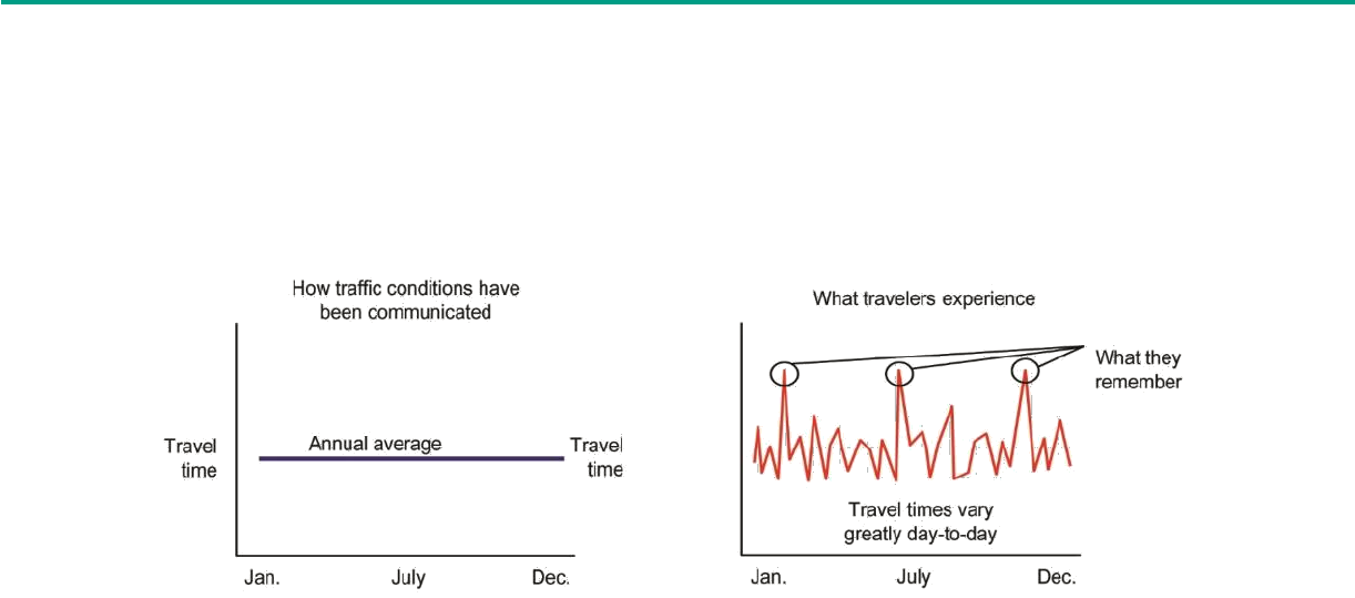
HIGHWAY SAFETY BENEFIT COST ANALYSIS GUIDE CHAPTER 4

captures the change in recurring travel time. As shown in Figure 5, the use of average travel

time may not realistically represent actual travelers’ experiences.

Average travel time may not realistically represent

actual travelers’ experiences.

Figure 5. Chart. Recurring travel time measurement versus actual traveler

experience.

(26)

Significant research and analyses have been performed on the effects of nonrecurring travel

time delay caused by factors such as crashes, special events, weather, and construction work

zones. Research completed as part of the Transportation Research Board’s (TRB) Second

Strategic Highway Research Program (SHRP2) and other Federal and State efforts have shown

the amount of delay caused by nonrecurring congestion is substantial. Omitting this measure

from transportation BCA may severely understate potential project benefits. This section

describes several methods for evaluating travel time reliability.

Travel time reliability measurement seeks to quantify the variability in travel times caused by

nonrecurring and recurring congestion sources to better estimate the full distribution of travel

times experienced by the system users. Transportation researchers have developed several

performance measures and indices to help quantify reliability impacts.

Table 13 briefly defines each reliability measure and Figure 6 provides an example graphic to

illustrate these measures empirically. Many of these measures are based on an analysis of the

distribution of travel times for a segment or facility. For some measures, there are multiple

definitions based on SHRP2 reliability research.

(27)

For example, the Planning Time Index and

Buffer Index are best estimated using the median travel time; however, median travel time may

not be readily available. In such cases, the analyst may need to substitute average travel time for

median travel time. The Failure/On-Time metrics may be based on either travel time or speed

brackets. Either may be appropriate, depending on the data available.

HIGHWAY SAFETY BENEFIT COST ANALYSIS GUIDE CHAPTER 4

This Guide uses buffer time to estimate the impact of crash reductions (or increases) on

reliability. Buffer time is the amount of extra time that most travelers add to their average

travel time to ensure a certain level of on-time arrival. Figure 6 shows buffer time as the

difference between the mean travel time (TT

) and the travel time at 95 percent on-time arrival

assurance (TT

). Whether expressed as a percentage or in minutes, it represents the extra

time a traveler should allow to arrive on-time for 95 percent of all trips. A simple analogy is

that a traveler who uses a 95 percent reliability indicator would be late only one weekday per

month. The standard deviation of travel time approximates the mean buffer time travelers

would need to meet their individual on-time requirements given their experience with the

network performance. As such, the change in the standard deviation of travel time

approximates the change in the mean buffer time.

Table 13. Reliability performance measures.

(27)

Performance Metric

Definition

Units

Planning-Time Index

• 95

percentile Travel Time Index (95

percentile

travel-time divided by the free-flow travel time),

normalized by the average travel time.

• The difference between the 95

percentile travel

time and the median travel time, normalized by

the median travel time.

None

Buffer Index (BI)

• The difference between the 95

percentile travel

time and the average travel time, normalized by

the average travel time, often shown for 80%,

85%, or 90% as well.

• The difference between the 95

percentile travel

time and the median travel time, normalized by

the median travel time, often shown for 80%,

85%, or 90% as well.

Percent

Failure/On-Time

Measures

• Percent of trips with travel times less than 1.1 *

Median Travel Time or 1.25 * Median Travel

Time.

• Percent of trips with space mean speed less than

50 mph, 45 mph, or 30 mph.

Percent

Percentile Travel-

Time Index

• 80

percentile travel time divided by the free-

flow travel time.

None

Skew Statistic

• The ratio of (90

percentile travel time minus

the median) divided by (the median minus the

percentile).

None

Misery Index (Modified)

• The average of the highest five percent of travel

times divided by the free-flow travel time.

None

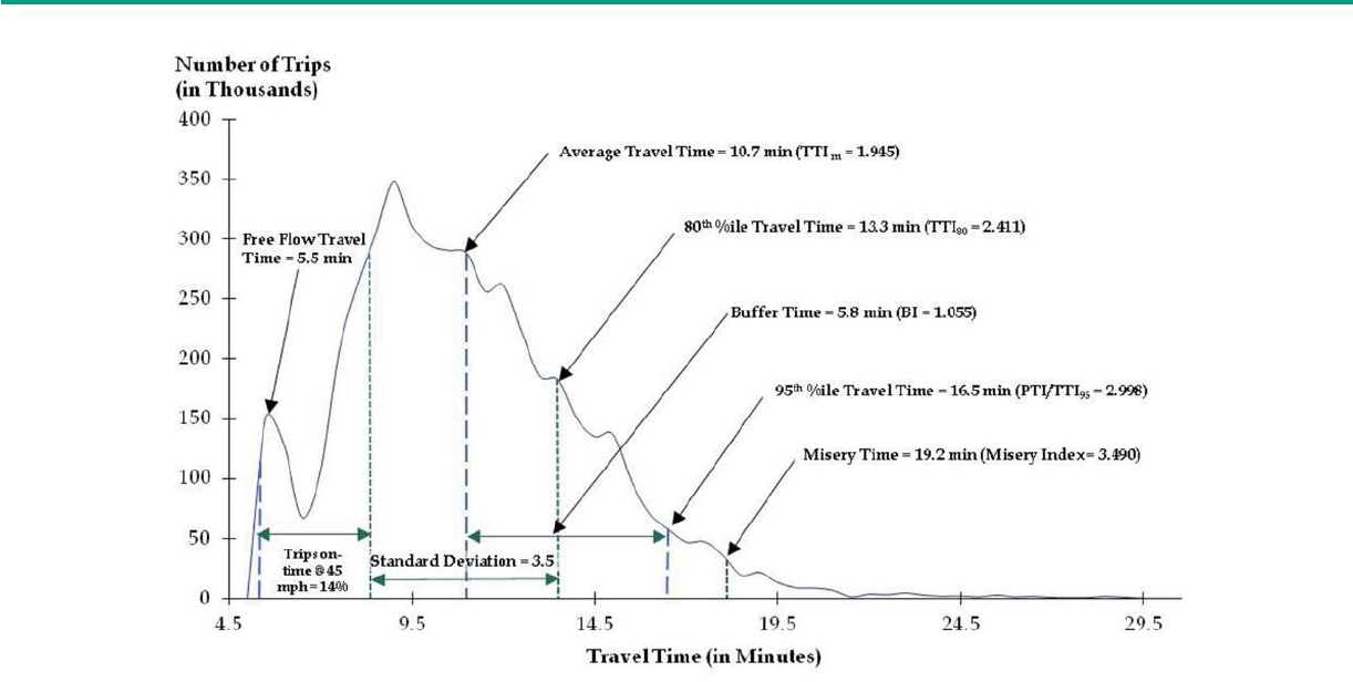
HIGHWAY SAFETY BENEFIT COST ANALYSIS GUIDE CHAPTER 4

Figure 6. Chart. Relationship of travel time measures and reliability.

(28)

This Guide and Tool use buffer time to estimate the

impact of crash reductions (or increases) on reliability.

4.3.1 Value of Travel Time Reliability

Projects that improve safety also improve reliability by reducing the number and severity of

crashes. To the extent that crash reductions improve network performance, travelers can

reduce the buffer time, realizing benefits related to time savings. To monetize estimates of

travel time reliability, a value of time measure is applied to the travel time reliability savings

measure. The analyst can monetize the time savings using the preferred value of time (either

local value of time or national values such as those in Table 10).

This type of analysis applies to the evaluation of travel time reliability for existing transportation

facilities. This method is not as useful as a predictive tool. Further, sufficient data are required

to support the estimation of the travel time distributions. In addition, transportation projects

may have a direct benefit on travel time reliability, beyond the indirect benefit of crash

reductions. As such, the analyst should seek to estimate and include these additional direct

benefits in the BCA as needed.

HIGHWAY SAFETY BENEFIT COST ANALYSIS GUIDE CHAPTER 4

Transportation projects may have a direct benefit on travel

time reliability, beyond the indirect benefit of crash

reductions or increases.

4.3.2 Data Sources for Travel Time Reliability

Travel time distributions are obtained from modern real-time vehicle to infrastructure (V2I)

travel data collection, long-term data archive systems, multiple manual data collection and

monitoring activities, or modeling efforts using multiple scenarios representing expected traffic

conditions. The analyst then multiplies the net change in the standard deviation in minutes of

travel time by the number of facility users. This calculation provides a temporal measure of

travel time reliability savings which can be monetized in a BCA.

The analyst should ensure that the dataset used to estimate the distribution of travel times is

sufficiently robust to capture travel times during a representative sampling of conditions. This

may require six months, for relatively simple cases, to multiple years’ worth of continuous data,

where an elevated level of confidence in analysis results is required. For a BCA, the analyst

should consider the overall project budget and level of effort desired before undertaking a

travel time reliability study that involves months or years of effort.

4.4 VEHICLE OPERATING COSTS

Change in net vehicle operating cost is a common measure used for transportation projects. A

BCA typically breaks out vehicle operating cost into fuel use and nonfuel use categories;

although, they may be combined as a single measure. Nonfuel use costs typically include vehicle

maintenance, insurance, and depreciation, but do not include vehicle registration and taxes

because economists consider these transfers. Benefits attributable to lower vehicle operating

cost are usually not a major component of a project's overall benefit.

Estimation of vehicle operating cost is often based on simple valuations applied directly to

vehicle miles traveled (VMT). Any net change in total VMT or roadway speed attributable to a

project alternative will affect fuel use. For simple analysis, the BCA applies a static rate of

average fuel use (gallons per VMT) to any net change in VMT to estimate the net change in fuel

use. The BCA then applies a benefit value (cost per gallon of fuel exclusive of fuel taxes) to the

change in the number of gallons of fuel consumed. The federal government anticipates future

year vehicle fleets to have greatly improved fuel use rates. Since estimated fuel use rates can

differ substantially based upon the year of analysis, practitioners are encouraged to use fuel

rates appropriate to that year.

(29)

HIGHWAY SAFETY BENEFIT COST ANALYSIS GUIDE CHAPTER 4

For nonfuel operating costs (e.g., maintenance, tires, tolls, lease, and financing), the BCA can

estimate the benefit values through VMT and change in VMT. Like fuel use rates, this benefit

value may be sensitive to the forecast year of analysis; however, nonfuel vehicle operating costs

are usually not sensitive to differences in operating conditions (e.g., travel speeds).

For highway safety BCA, it is necessary to relate the change in safety performance to a change

in fuel use as the project may or may not impact VMT. The NHTSA report, The Economic and

Societal Impact of Motor Vehicle Crashes, provides values of increased fuel use per crash by crash

severity and roadway facility type.

(11)

Chapter 6 provides further details on applying this method.

This Guide focuses on reductions in fuel use

that result from crash reductions.

4.4.1 Value of Vehicle Operating Costs

To monetize fuel-related benefits, apply the cost per gallon of fuel, exclusive of fuel taxes, to

the change in fuel use. Analysts can obtain estimates of fuel costs from websites such as the US

Energy Information Administration.

(30)

To monetize nonfuel vehicle-use benefits, apply the average vehicle operating cost per mile to

the change in VMT. This Guide does not include nonfuel vehicle-use benefits in the highway

safety BCA because most safety projects do not impact the VMT. Specifically, there is limited or

no induced demand so the expected change in VMT would be the same for the base and

alternative conditions.

The vehicle operating cost per mile varies by type and age of vehicle. Even within light duty

vehicles, there are substantial variations in vehicle operating cost per mile due to differences in

vehicle weight, design, fuel type, and other factors. The Benefit-Cost Analysis Guidance for

TIGER and INFRA Applications recommends a 2016 value of $0.40 per mile for light duty

vehicles and $0.96 per mile for heavy duty vehicles. The light duty vehicle operating cost is

based on an average sedan and costs such as gasoline, maintenance, tires, and depreciation,

assuming an average of 15,000 miles driven per year. The value omits other ownership costs

that are mostly fixed or transfers (insurance, license, registration, taxes, and financing charges).

The heavy-duty vehicle operating cost includes fuel costs, truck/trailer lease or purchase

payments, repair and maintenance, truck insurance premiums, permits and licenses, and tires.

The value omits tolls (transfers) and driver wages and benefits, which are included in the value

of travel time savings.

HIGHWAY SAFETY BENEFIT COST ANALYSIS GUIDE CHAPTER 4

4.4.2 Data Sources for Vehicle Operating Costs

The Benefit-Cost Analysis Guidance for TIGER and INFRA Applications is updated periodically

providing the latest USDOT-approved values for vehicle operating cost. The 2017 version

provides 2016 values based on data from the following sources:

• American Automobile Association, Your Driving Costs – 2016 Edition (2016),

http://exchange.aaa.com/automotive/driving-costs/#.WVZdF02oupp.

(31)

• American Transportation Research Institute, An Analysis of the Operational Costs of

Trucking: 2016 Update (2016), http://atri-online.org/wp-content/uploads/2016/10/ATRI-

Operational-Costs-of-Trucking-2016-09-2016.pdf.

(32)

These values are updated annually, which is typically more frequent than the USDOT BCA

guidance. The analyst can use the source information or use the CPI to update the DOT values

between publication years.

(33)

For example, to update 2016 values to 2017, multiply by 1.6154

(i.e., 2.1 percent average annual CPI in 2017 divided by 1.3 percent average annual CPI in 2016).

4.5 EXTERNALITIES

One of the more challenging areas of BCA is the treatment and valuation of externalities (non-

user costs) related to transportation projects. Economists define an externality as the

uncompensated impact of one person's actions on the well-being of a bystander. In the case of

transportation investments, "bystanders" are the non-users of the project.

Externalities include uncompensated impacts on bystanders.

Examples of externalities include the following:

• Changes in air emissions (e.g., criteria pollutants regulated by the Clean Air Act).

• Noise impact (i.e., increases or decreases in noise levels).

• Construction impacts (e.g., degradation in roadway level of service on surrounding

neighborhoods).

• Impacts to natural habitats, wetlands, and streams.

• Permanent property value impacts.

When the impact benefits the non-user, economists refer to it as a positive externality. When

the impact is adverse, economists refer to it as a negative externality. Often, the BCA focuses

on negative externalities. Negative externalities include the undesirable effects of a project on

air and water quality, noise and construction disruptions, and other community or aesthetic

HIGHWAY SAFETY BENEFIT COST ANALYSIS GUIDE CHAPTER 4

impacts as described. Positive externalities, however, also exist. For example, a project may

serve to reduce air or noise pollution from previously existing or projected levels.

Transportation agencies generally analyze a project’s environmental impact (including

externalities) through environmental studies required by the NEPA as well as other State and

local environmental compliance laws. This is particularly the case for larger projects where the

agency must prepare an Environmental Impact Statement (EIS) or Environmental Assessment

(EA). The EIS or EA generally quantifies the project’s impact to air quality, noise levels, and the

natural environment such as loss of wetlands or habitat for threatened and endangered species.

Analysts can use NEPA studies to quantify the impact of externalities for use in a BCA.

Transportation agencies should closely coordinate NEPA studies and BCA to the extent

possible. Where possible, the analyst should utilize the analysis completed through the NEPA

process to evaluate the cost to mitigate natural environmental impacts (e.g., wetland or habitat

loss). Analysts may also use environmental impacts described in the NEPA study to qualitatively

evaluate and compare alternatives. The BCA can utilize broader impact estimates to more

accurately estimate project costs and benefits (e.g., estimates of air quality impacts from a larger

program of safety improvements implemented on a statewide level).

Analysts can use the results of NEPA studies to

quantify the impact of externalities for use in a BCA.

Emissions are a common externality monetized for transportation projects. The inclusion of

emissions estimates in BCA is particularly important when transportation agencies prioritize

projects in competition for several types of funding (e.g., Safety, Operations, or Congestion

Mitigation, and Air Quality (CMAQ) funds), or the project is considered in an air quality

nonattainment area.

The Clean Air Act requires the Environmental Protection Agency (EPA) to set National

Ambient Air Quality Standards (40 CFR part 50) for pollutants considered harmful to public

health and the environment. The Clean Air Act identifies two types of national ambient air

quality standards: primary and secondary. Primary standards provide public health protection,

including protecting the health of "sensitive" populations such as asthmatics, children, and the

elderly. Secondary standards provide public welfare protection, including protection against

decreased visibility and damage to animals, crops, vegetation, and buildings.

The EPA has set National Ambient Air Quality Standards for six principal pollutants, which are

called "criteria" air pollutants. Periodically, the standards are reviewed and revised. The current

standards are listed below. A BCA often includes one or more of these pollutants depending on

the concerns of the local region. Units of measure for the standards are parts per million (ppm)

by volume, parts per billion (ppb) by volume, and micrograms per cubic meter of air (µg/m

HIGHWAY SAFETY BENEFIT COST ANALYSIS GUIDE CHAPTER 4

• Hydrocarbons (HC)/Reactive Organic Gases (ROG).

• Nitrous Oxide (NOx).

• Carbon Monoxide (CO).

• Carbon Dioxide (CO2).

• Particulate Matter (PM10) or Fine Particulate Matter (PM2.5).

• Sulfur Dioxide (SO2).

4.5.1 Value of Emissions

The NHTSA report, The Economic and Societal Impact of Motor Vehicle Crashes, provides

monetized values for select emissions per crash by crash severity and roadway facility type.

(11)

These emissions include volatile organic compounds (VOCs), but do not include PM10 or CO.

PM10 is not included because virtually all the adverse health impacts from PM arise from fine

particulates, defined as the fraction that is less than 2.5 microns in diameter (hence the notation

PM2.5). CO is not included because at current exposure levels, there is no evidence that CO

causes any adverse health impacts. Table 14 through Table 16 present the NHTSA-developed

emissions values for five facility types, converted to 2017 dollars using the CPI.

This Guide focuses on emissions reductions that result from

crash reductions. Analysts should seek other data and tools

to estimate direct emissions benefits.

Table 14. Estimated value of net emissions per fatal crash (2017 dollars).

(11)

Facility Type

2.5

VOC

Total

Emissions

Urban Interstate /

Expressway

$827.90

$197.59

$895.53

$70.79

$23.61

$2,015.41

Urban Arterial

$213.66

$50.27

$133.83

$18.09

$3.99

$419.84

Urban Other

$16.37

$3.95

$8.92

$1.41

$0.27

$30.92

Rural Interstate / Principal

Arterials

$124.60

$59.72

$178.65

$10.38

$2.44

$375.79

Rural Other

$15.47

$6.28

$17.54

$1.28

$0.28

$40.84

Average for All Road Types

$159.48

$44.36

$159.17

$13.53

$3.82

$380.36

HIGHWAY SAFETY BENEFIT COST ANALYSIS GUIDE CHAPTER 4

Table 15. Estimated value of net emissions per injury crash (2017 dollars).

(11)

Facility Type

2.5

VOC

Total

Emissions

Urban Interstate /

Expressway

$174.91

$41.74

$189.15

$14.98

$4.99

$425.77

Urban Arterial

$47.38

$11.14

$29.16

$4.02

$0.88

$92.57

Urban Other

$7.18

$1.72

$3.76

$0.62

$0.12

$13.41

Rural Interstate / Principal

Arterials

$22.98

$11.02

$33.05

$1.94

$0.45

$69.43

Rural Other

$3.93

$1.59

$4.38

$0.32

$0.07

$10.29

Average for All Road Types

$34.29

$9.40

$33.45

$2.92

$0.81

$80.87

Table 16. Estimated value of net emissions per PDO crash (2017 dollars).

(11)

Facility Type

2.5

VOC

Total

Emissions

Urban Interstate /

Expressway

$148.76

$35.51

$160.61

$12.67

$4.24

$361.79

Urban Arterial

$28.71

$6.75

$18.34

$2.41

$0.53

$56.75

Urban Other

$4.33

$1.05

$2.25

$0.36

$0.08

$8.06

Rural Interstate / Principal

Arterials

$23.38

$11.21

$33.38

$1.91

$0.46

$70.34

Rural Other

$3.28

$1.34

$3.59

$0.28

$0.06

$8.55

Average for All Road Types

$27.16

$7.70

$27.85

$2.29

$0.66

$65.67

When an agency cannot quantify the dollar value of an externality, they may choose to deal

with it on an as-needed qualitative basis. If the measurable net benefits of a project are highly

positive, decision makers may tolerate minor unquantified externalities from an economic

standpoint, even if the agency perceives the externalities to be negative. On the other hand, if

the net benefits are very low, then the existence of significant unquantified negative

externalities may tip the economic balance against the project. An example of this could include

negative impacts to low-income and minority populations that live near the project location.

The project could impact these populations through increases in air pollution, noise, or traffic.

HIGHWAY SAFETY BENEFIT COST ANALYSIS GUIDE CHAPTER 4

Analysts may deal with externalities on a qualitative

basis if they cannot quantify the dollar value.

It may not be easy to monetize quality of life measures or other potentially controversial

measures. The BCA can include such items through qualitative presentations. These types of

externalities become important if the monetized present value of benefits do not exceed or

only barely exceed the monetized present value of costs.

4.5.2 Data Sources for Emissions

Emissions may represent one of the most complex measures to estimate in BCA. This is due to

the many variables that determine the appropriate emission rates. Most emissions estimations

are based on an application of an emissions rate on a per VMT basis. Depending on the

emissions category, the appropriate emissions rate to apply may be sensitive to numerous

factors, including the following:

• Year of the analysis (i.e., the EPA anticipates future year vehicle fleets to produce fewer

emissions in many categories).

• The mix of gasoline and diesel vehicles in the regional fleet.

• Vehicle speeds.

• The number of cold starts.

• The mix of vehicles in the regional vehicle mix (e.g., autos, light trucks, medium-duty

trucks, heavy-duty trucks, etc.).

• Regional weather patterns/climate and other considerations.

Given these many variables impacting emissions rates, analysts should obtain rates using existing

emissions analysis tools, calibrated to the individual region or derived from previously

conducted regional analysis. Therefore, analysts should use caution when applying emissions

rates derived from other regions or based on averages among different regions. This Guide

does not provide detailed estimates of emissions rates by region, but does provide a method

for quantifying and monetizing emissions based on the expected change in crashes (refer to

Chapter 6).

4.6 CHAPTER SUMMARY

Chapter 4 describes various types of project benefits included in a highway safety BCA. The

safety benefits result in direct and indirect impacts. Direct safety benefits are the expected

reduction in crash frequency and severity. Indirect benefits include reductions in travel time,

HIGHWAY SAFETY BENEFIT COST ANALYSIS GUIDE CHAPTER 4

vehicle operating costs, and emissions resulting from fewer crashes. Each section provides

default values to monetize project benefits.

Key Takeaways from Chapter 4:

• Safety benefits are derived from a change in safety performance (i.e., change in the

frequency and/or severity of crashes), which may result in direct and indirect benefits.

• Direct safety benefits include the reduction in crash frequency and/or severity.

• To monetize direct safety benefits for a BCA, multiply the estimated change in long-

term average crashes by the average comprehensive crash cost.

• Comprehensive crash costs (or societal crash costs) are generally most appropriate for

monetizing the value of crashes as they capture all impacts resulting from crashes.

• Indirect safety benefits include reductions in travel time, vehicle operating costs, and

emissions resulting from fewer crashes.

• This Guide does not consider direct operational and environmental impacts such as

reductions in recurring delay.

• The NHTSA report, The Economic and Societal Impact of Motor Vehicle Crashes, provides a

method to estimate and monetize the indirect safety benefits.

(11)

HIGHWAY SAFETY BENEFIT COST ANALYSIS GUIDE CHAPTER 4

THIS PAGE IS INTENTIONALLY LEFT BLANK

HIGHWAY SAFETY BENEFIT COST ANALYSIS GUIDE CHAPTER 5

5. PREPARING FOR A BCA

The BCA process begins with the development of a base condition. This serves as a basis for

comparing other project alternatives. In preparing for a BCA, it is also important to establish

the analysis period, consider the need to evaluate uncertainty, and select a discount rate. This

chapter describes these components of preparing for a BCA. The chapter also describes

potential challenges and opportunities to overcome these challenges in BCA.

Chapter 5 At-A-Glance

Chapter 5 is divided into six sections:

• Section 5.1 describes the purpose and importance of establishing the base condition.

• Section 5.2 discusses the purpose of setting an analysis period for the BCA.

• Section 5.3 defines uncertainty and describes the purpose of evaluating uncertainty in

BCA.

• Section 5.4 introduces the concept of discounting and appropriate discount rates.

• Section 5.5 identifies challenges and opportunities to overcome challenges in BCA.

• Section 5.6 provides a summary of the chapter.

5.1 DEVELOPING THE PROJECT BASE CONDITION

Critical to a successful BCA is development of the project base condition. The base condition is

the project alternative against which the analyst evaluates other project alternatives (i.e., does

the project alternative provide net benefits compared with the base condition). This is often the

existing condition (or “no-build” or “do nothing” alternative), representing the continued

operation of the existing transportation facility under good management practices with minor

or no capital investments.

Accurately defining the base condition is critical to

the success of a BCA.

The definition of the base condition can have significant impacts on the BCA; therefore, it is

important to carefully define values such as existing and future traffic volumes. Further, the

estimated safety performance of the base condition is the basis for highway safety BCA and

related decision-making. As such, it is imperative that analysts use a reliable method to estimate

the safety performance of the base condition. The following are several factors to consider in

selecting an appropriate method to estimate the safety performance of the base condition:

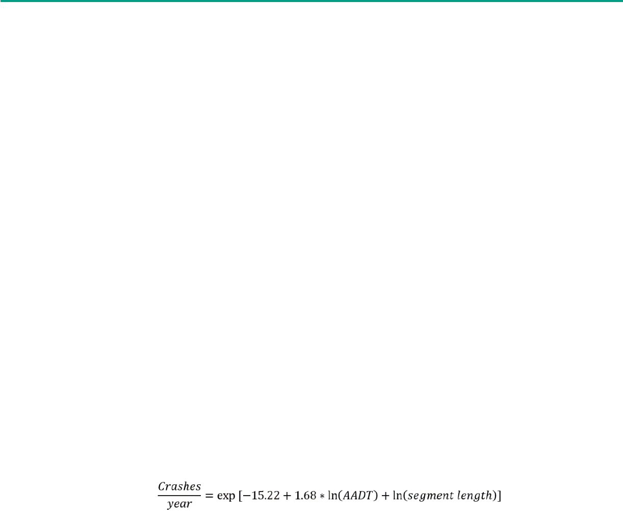
HIGHWAY SAFETY BENEFIT COST ANALYSIS GUIDE CHAPTER 5

• Data availability (years of crash, roadway, and traffic data).

• Annual fluctuation in observed crashes.

• Changes in geometric or traffic control characteristics.

• SPF availability and reliability.

• Potential for changes in traffic volume.

In addition to the factors listed above, analysts should consider the trade-off between the

reliability of the method and the resources needed to conduct the analysis.

The Highway Safety Manual provides three methods to estimate the safety performance of a

base condition: observed, predicted, and expected crashes.

(7)

Observed crashes are the historical crashes reported for an existing site. For

example, if there were 15 reported crashes at an existing intersection over the last five

years, then the observed number of crashes is 15 (or 3.0 crashes per year on average).

Using the observed crash frequency assumes the observed crashes before the project

represent the long-term future safety performance in the absence of projects or other

changes to the site. This assumption does not account for year-to-year changes in

conditions at the location of interest (e.g., changes in traffic, weather, crash reporting,

road conditions, land use, vehicle fleet, and driver behavior).

Predicted crashes are based on SPFs, which are mathematical models used to predict

mean crash frequency based on exposure for a given facility type. For example, if the

SPF for a given facility type is represented by Figure 7, and the location of interest is 2.5

miles with 7,500 vehicles per day, then the predicted number of crashes is 1.99 per year

[exp(-15.22 + 1.68*ln(7500) + ln(2.5)]. If the traffic volume is expected to change during

the analysis period, consider using the average value to represent the traffic volume.

Figure 7. Equation. Example SPF.

Using the predicted crash frequency assumes the SPF prediction is representative of

future safety performance. This method accounts for changes in traffic volume and can

incorporate adjustment and calibration factors to account for changes in geometrics and

general time trends; however, it requires jurisdiction-specific SPFs or SPFs calibrated to

local conditions. Further, the SPF should be developed using data for similar sites at

which the countermeasure of interest has not been implemented. This method does not

HIGHWAY SAFETY BENEFIT COST ANALYSIS GUIDE CHAPTER 5

consider historical crash data for any specific location of interest in estimating future

safety performance.

Expected crashes are based on the weighted average of observed and predicted

crashes using the Empirical Bayes method. The weight placed on the predicted crashes is

based on the statistical reliability of the SPF as well as the magnitude of the predicted

crash frequency. Using the expected crash frequency assumes the combined observed

and predicted crash frequency is representative of future safety performance. This

method accounts for changes in traffic volume, regression-to-the-mean, and can

incorporate adjustment and calibration factors to account for changes in geometrics and

general time trends. This method requires jurisdiction-specific SPFs or SPFs calibrated to

local conditions. Further, the SPF should be developed using data for similar sites at

which the countermeasure of interest has not been implemented. If the traffic volume is

expected to change during the analysis period, consider using the average value to

represent the traffic volume when using SPFs to estimate predicted crashes.

Table 17 provides an overview of the characteristics associated with the three methods for

estimating the safety performance of the base condition. This table can help determine when

each method is (or is not) appropriate for estimating the safety performance of the base

condition. The following are additional insights to help select an appropriate method:

• Research has shown the observed crashes may overestimate the crashes for the base

condition, particularly when there is a high degree of annual fluctuation in the observed

crashes.

(4)

• If a calibrated SPF is available, the predicted or expected crashes can help to normalize

annual fluctuations in observed crashes and account for changes in traffic volume.

• The observed crashes may provide a reasonable estimate when there are several years

of historical crash data and limited fluctuation in crashes from year to year.

• Expected crashes are typically more reliable than predicted crashes, assuming the

observed crashes for the base condition are applicable to future conditions.

• Predicted crashes are most appropriate when the observed crashes are not a good

approximation of future conditions.

• Observed crashes are not a good approximation of future conditions when there are

major changes to the land use, traffic operations, or facility type. For example, if a

project includes road widening from two to four lanes, then the observed crash

frequency under existing conditions (i.e., two-lane facility) would not represent the

future safety performance under future conditions (i.e., four-lane facility).

Refer to the Highway Safety Manual for further discussion of methods to estimate the safety

performance of base conditions.

(7)

HIGHWAY SAFETY BENEFIT COST ANALYSIS GUIDE CHAPTER 5

Table 17. Overview of methods to estimate safety performance of base condition.

Characteristics

Observed

Crashes

Predicted

Crashes

Expected

Crashes

Method limited by large degree of annual

crash fluctuation

●

Reasonable when there are several years of

historical crash data with limited fluctuation

●

Appropriate to normalize annual crash

fluctuations

●

Applicable when facility type changes due

to countermeasure

●

Requires calibrated SPF

●

Accounts for traffic volume changes

●

Note: -- indicates not applicable.

5.2 SETTING AN ANALYSIS PERIOD

BCA attempts to capture the comprehensive costs and benefits that result from a project over

the lifecycle and within a defined analysis period (e.g., 10- or 20-year time horizon). In setting an

analysis period, it is necessary to define an appropriate timeframe to allow for a meaningful

analysis and a fair comparison of alternatives. FHWA recommends that the analysis period

include the initial construction and at least one subsequent rehabilitation action for each

alternative.

(8)

Using BCA, the analyst calculates the lifecycle costs and benefits of each alternative over the

same analysis period. When the service life is different among project alternatives, the analyst

should standardize the service life comparisons. One method to standardize the service life

comparisons is to use the least common multiple of the service lives. For example, if alternative

1 has a service life of four years and alternative 2 has a service life of eight years, then the least

common multiple is an analysis period of eight years. In this case, the analyst would estimate the

initial cost to implement each alternative and assume one replacement of alternative 1 at the

end of the fourth year.

The analyst should standardize the analysis period to

ensure a fair comparison of alternatives.

Within the analysis period, alternatives may have different maintenance or rehabilitation

requirements at various times. For example, the cost components for a given project may

include safety-related hardware, software, and operations and maintenance costs. For

HIGHWAY SAFETY BENEFIT COST ANALYSIS GUIDE CHAPTER 5

alternative 1, the hardware has an estimated 10-year service life and the software requires

updating every five years. For alternative 2, the hardware has an estimated 15-year service life

and the software requires updates every five years. An appropriate analysis period should

account for the difference in service life for the hardware. Using the least common multiple of

the service lives, a potential analysis period is 30 years. For alternative 1, this would include the

initial cost and two replacements (i.e., replacement in years 10 and 20). For the second

alternative, this would include the initial cost and one replacement (i.e., replacement in year

15). Both alternatives would include the initial software cost and five replacements (i.e.,

replacements in years 5, 10, 15, 20, and 25). In this example, the 30-year analysis period

provides a fair comparison between alternatives with different hardware lifespans.

As another example, consider the cost of installing a traffic signal or constructing a roundabout

at an existing two-way stop-controlled intersection. If the expected service life of the traffic

signal is 10 years and the expected service life of the roundabout is 25 years, then a common

multiple is a 50-year analysis period.

5.3 EVALUATING UNCERTAINTY

Transportation agencies evaluate and manage uncertainty associated with transportation

investments by attempting to measure uncertainty. Analysts can measure many uncertainties by

quantifying the probability of occurrence and impact of an event. Analysts identify and evaluate

uncertainty by answering three questions:

• What can happen? Uncertainties affect the BCA results. These uncertainties include

changes in initial construction estimates or future rehabilitation cost overruns,

inaccurate facility service life costs, or variations in traffic volumes that differ significantly

from forecasts.

• How likely is it to happen? Some uncertainties are more likely to occur than others.

For instance, it may be that the transportation agency has an excellent understanding of

project costs and unlikely to have construction cost overruns.

• What are the consequences of it happening? In some cases, an input variable may

be subject to significant variability, but any given occurrence (within a realistic range)

would not substantially affect the economic justification for the project. For instance,

the price of a paving material may be subject to large swings, but the benefits of an

alternative using that material may be sufficiently large to maintain the alternative as the

preferred alternative even if the paving material price doubles. In other cases, there may

be little likelihood that an event will occur (such as an earthquake), but its occurrence

would have major consequences unless the transportation agency takes certain

precautions in the project’s design.

HIGHWAY SAFETY BENEFIT COST ANALYSIS GUIDE CHAPTER 5

Assessing uncertainty helps analysts to answer these questions and determine if efforts to

mitigate uncertainty is cost-effective. The traditional means by which analysts have evaluated

uncertainty is through sensitivity and probabilistic analyses. The following sections describe

methods to evaluate uncertainty.

5.3.1 Sensitivity Analysis

The traditional means by which analysts have evaluated uncertainty is through sensitivity

analysis. A sensitivity analysis provides a method to alleviate concerns related to the quality or

credibility of data or specific inputs. In a typical sensitivity analysis, the value of an input variable

identified as a significant potential source of uncertainty is changed (either within some

percentage of the initial value or over a range of reasonable values) while all other input values

are held constant, and the amount of change in analysis results is noted. This sensitivity process

is repeated for other input variables for which uncertainty has been identified. The input

variables may then be ranked per the effect of their variability on BCA results.

In highway safety analysis, analysts can consider the certainty (or uncertainty) of the estimated

change in crashes by computing a confidence interval. The analyst would have more certainty in

the estimated change in crashes, and resulting benefits, as the width of the confidence interval

decreases. For example, if the CMF is 0.75 with a 95 percent confidence interval of 0.41 to

1.09, then there is a 95 percent chance that the true CMF value is between 0.41 and 1.09. If the

confidence interval includes 1.0, as in this example, then the countermeasure may result in a

reduction, no change, or an increase in crashes. To incorporate this measure of uncertainty in

highway safety BCA, the analyst could use the end points of the confidence interval (e.g., 0.41

and 1.09) in addition to the point estimate of the CMF when estimating the change in crashes

and resulting benefits. Refer to FHWA’s guide, Quantifying Safety in the Roadway Safety

Management Process, for further discussion on estimating the confidence interval.

(34)

5.3.2 Probabilistic Analysis

Continued advances in computing power permit the practice of probabilistic-based uncertainty

analysis, most often through a method known as Monte Carlo simulation. In Monte Carlo

simulation, the analyst assigns an appropriate probability distribution (based on expert opinion,

historical data, and other information) to each of the input variables subject to uncertainty in

the economic analysis. The Monte Carlo simulation draws random samples from the probability

distributions for each input, runs the selected input values through the BCA formula to

calculate a discrete economic result, and then repeats this process numerous times. The

results, based on the randomly selected input values, produce an average BCA measure and an

associated probability distribution to indicate the range of potential outcomes of the BCA.

Refer to the Economic Analysis Primer for further details on probabilistic analysis and other

fundamental economic analysis concepts.

(8)

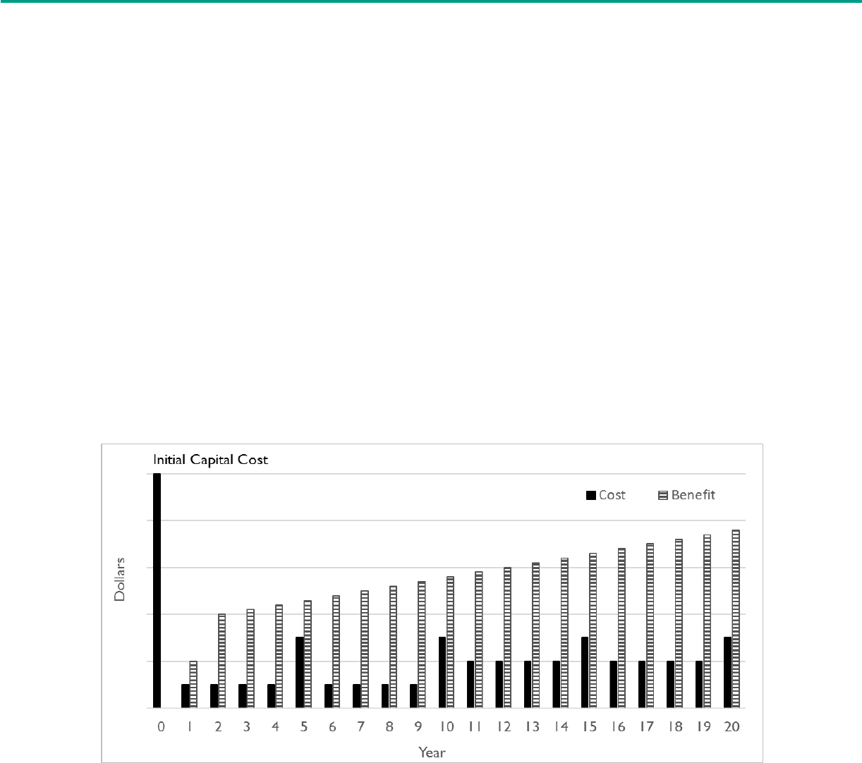
HIGHWAY SAFETY BENEFIT COST ANALYSIS GUIDE CHAPTER 5

5.4 DISCOUNTING

The most basic economic questions that people face in their personal and business lives involve

the tradeoffs between dollars earned, spent, or invested today and those dollars they hope to

earn, spend, or invest in the future. Project lifecycle evaluation is important for transportation

projects as these activities can be long-lived and require initial and periodic capital investments,

as well as ongoing materials and maintenance expenditures.

Figure 8 shows an example distribution of project costs and benefits over time. These typically

include initial construction costs (year 0), annual maintenance costs (years 1 to 4, 6 to 9, 11 to

14, and 16 to 19), and periodic rehabilitation and reconstruction costs (years 5, 10, 15, and 20).

The periodic rehabilitation and reconstruction costs are necessary if the analysis period is

longer than the expected service life of the project. Benefits may grow rapidly in the first few

years after implementation and level out in later years as the public becomes accustomed to the

project. The assumption of increasing benefits, as shown in the figure, does not necessarily

apply to all projects, but depends on which strategy the agency implements. Some strategies,

such as pavement markings or enhanced surface friction, may have the greatest benefits in the

first few years after implementation, then lose effectiveness due to degradation over time.

Figure 8. Chart. Time series of costs and benefits (in constant dollars).

(8)

A dollar that an agency spends or earns in the future is almost always worth less to them today

than a dollar they spend or earn now. The BCA quantifies the changing value of the dollar to

enable meaningful comparisons of multiyear dollar streams. Two separate and distinct factors

account for why the value of a dollar, as seen from the present, diminishes over time. These

factors are inflation and the time value of resources, also referred to as “discounting.”

HIGHWAY SAFETY BENEFIT COST ANALYSIS GUIDE CHAPTER 5

Two separate and distinct factors account for why the present

value of a dollar diminishes over time: inflation and discounting.

5.4.1 Inflation

In the case of economic analysis of investments by a public agency, the suggested practice is to

forecast lifecycle costs and benefits of a project without inflation (i.e., in real or base year

dollars). Inflation is hard to predict, particularly in the long-term for a project meant to be in

service for decades. More importantly, if the BCA adds inflation to the calculation of benefits

and costs projected for future years, it will only have to be removed again before these benefits

and costs can be compared in the form of dollars in any given base year.

Inflation is generally not considered in BCA.

5.4.2 Discounting

The application of the discount rate to future sums to calculate their present value is known as

"discounting.” Through discounting, the BCA can objectively compare different investment

alternatives based on their respective present values, even though each has a different stream of

future benefits and costs.

Figure 9 and Figure 10 provide the formulas for discounting. For example, if the discount rate is

3.0 percent, the discount factor (from Figure 10) for 10 years in the future is 0.744

(1/(1.03^10)). If the estimated benefit is $1000 for 10 years in the future, then the present value

(from Figure 9) is $744 (0.744 * $1000).

  



  







Figure 9. Equation. Standard formula for discounting.

where:

PV = present value at time zero (the base year).

r = discount rate.

t = time (year).

= amount of benefit or cost in year t.



  



Figure 10. Equation. Discount factor.

HIGHWAY SAFETY BENEFIT COST ANALYSIS GUIDE CHAPTER 5

Most transportation projects generate costs and benefits over their entire lifecycle. The BCA

should discount the entire series of costs and benefits to the present by multiple applications of

the PV formula for each applicable year of the lifecycle. Figure 11 provides the formula for this

calculation. These discounted values are then summed together (as represented by ∑) for each

year of the lifecycle analysis period (N years) to yield an overall present value.

 



  











Figure 11. Equation. Summation of discounted values.

5.4.3 Selecting a Discount Rate

Economic analysis should include real terms (i.e., using dollars and discount rates that do not

include the effects of inflation). The BCA can estimate the real discount rate by removing the

rate of inflation as measured by a general price index such as the CPI from a market or nominal

interest rate for government borrowing. The CPI is developed and maintained by the US

Department of Labor, Bureau of Labor Statistics. The CPI represents changes in prices of all

goods and services purchased for consumption by urban households. User fees (such as water

and sewer service) and sales and excise taxes paid by the consumer are also included. Income

taxes and investment items (like stocks, bonds, and life insurance) are not included. The

selected market rate for government borrowing should be based on government bonds with

maturities comparable in length to the analysis period used for the economic analysis. Real

discount rates calculated in this manner have historically ranged from just below zero percent

to five percent, which are the rates most often used by States for discounting highway

investments.

The 2017 Benefit-Cost Analysis Guidance for TIGER and INFRA Applications notes that

applicants should discount future benefits and costs to present values using a real discount rate

(i.e., a discount rate that reflects the opportunity cost of money net of the rate of inflation) of

seven percent, following guidance provided by the OMB in Circular A-94. Grant applicants may

also provide an alternative analysis using a real discount rate of three percent, for example. In

conducting BCA, the analyst should review the current OMB or State guidance on the

appropriate discount rate to use at the time of the analysis as this value will change over time

and location. OMB provides an annual memorandum providing appropriate discount rates. The

2017 rate for long-lived projects (meaning 10 years or more) is seven percent. Agencies may

perform a sensitivity analysis to determine how the discount rate impacts the results and use a

lower discount rate (e.g., three percent) if it better suits their needs.

Typical discount rates range from 3 to 7 percent.

HIGHWAY SAFETY BENEFIT COST ANALYSIS GUIDE CHAPTER 5

5.5 CHALLENGES AND OPPORTUNITIES

A BCA is a powerful, informative tool available to assist planners, engineers, and decision

makers. Nevertheless, public agencies may avoid or underutilize BCA due to misconceptions. In

some cases, agency personnel are skeptical about the accuracy of a BCA due to perceived

uncertainties in measuring or valuing costs and benefits. The analyst can often measure and

manage uncertainty where it exists, as described in section 5.3, Evaluating Uncertainty. It is

helpful to remember that sound economic analysis reduces uncertainty. Not performing the

analysis only serves to hide uncertainty from decision makers.

The following are opportunities related to BCA:

• Determine the cost-effectiveness of lifecycle costs, user benefits, and externalities.

• Provide documentation of decision-making and assumptions used in the analysis.

• Compare the economic effects of project alternatives.

• Make proactive decisions.

• Identify economically-efficient investments.

• Determine if a project or program should be undertaken and when.

• Determine which alternative and programs should be funded.

While there are several benefits related to BCA, transportation professionals should be aware

of challenges and limitations associated with BCA. Table 19 presents potential challenges and

opportunities to overcome those challenges in highway safety BCA.

Table 18. Frequently asked questions and answers for applying crash costs.

CHALLENGE

OPPORTUNITY

Data quality: A BCA can be data

intensive, and its accuracy and

precision depend on the quality of

the input data.

Analysts should take extra care in reviewing input data

to assure accuracy, and test the importance of

assumptions by running alternate scenarios and

performing sensitivity analysis.

Limited data capabilities: There

may be a lack of data capabilities to

estimate the long-term safety

performance of alternatives.

Efforts are underway to improve safety data

capabilities such as the availability of crash and traffic

volume data needed to estimate predicted and

expected crashes. Efforts are also underway in many

States to develop or calibrate SPFs.

Quantifying air emissions and

noise impacts: It may be difficult

to estimate air emissions and noise

impacts as these estimates can

The EIS or EA generally quantifies the project’s impact

to air quality, noise levels, and natural environment.

Analysts can use NEPA studies to quantify the impact

of externalities for use in a BCA. Analysts could also

HIGHWAY SAFETY BENEFIT COST ANALYSIS GUIDE CHAPTER 5

CHALLENGE

OPPORTUNITY

require field measurement and

specialized expertise.

use environmental impacts described in NEPA studies

to qualitatively evaluate and compare alternatives.

Uncertainty in assumed values:

When transportation professionals

collect data to support a BCA,

there may be uncertainty in

assigning engineering and economic

values to inputs and the resulting

outputs. The level of confidence in

the analytical results depends on the

relative certainty of the analysis

methods and underlying data.

Sensitivity analysis is an important part of economic

evaluation. Modern analysis tools give users the ability

to test several assumptions with little effort through

sensitivity analysis where key assumptions are

modified.

Ambiguous or inaccurate base

condition: If the analyst improperly

defines the base condition, then the

resulting comparison of alternatives

may be misleading.

The analyst can better define the base condition with

more detailed and reliable data. It is important to

define the base condition to represent the conditions

expected in the future if the project is not

implemented. Benefits accrue from the difference

expected from the implementation of a project

compared to the future conditions without the

project.

Accuracy in estimating

benefits: It is not always clear

whether prior research from other

locations or contexts is transferable

to a new project.

Benefit transfer is an economic analysis technique

utilized when local data are not available. As data

become available, the analyst can refine the inputs and

improve the accuracy of the results.

Transparency and

reproducibility: Analysis

techniques may lack transparency

and reproducibility in procedures

and results.

Modern analysis tools assist the analyst in producing

BCA results that are transparent, testable, and

reproducible.

Regulatory requirements: The

investment of Federal and some

State funds require agencies to

conduct a BCA prior to the

allocation of those funds. There may

be State regulatory requirements or

policies that force transportation

professionals to consider specific

criteria, costs, or benefits.

While the regulatory requirements may add to the

burden of the project development process, the BCA

results add value to the decision-making process.

HIGHWAY SAFETY BENEFIT COST ANALYSIS GUIDE CHAPTER 5

CHALLENGE

OPPORTUNITY

Lack of expertise and support:

There may be a lack of technical

expertise or institutional support

within transportation agencies to

conduct BCA or to perform a

rigorous analysis.

Great strides have been made by transportation

agencies to understand and utilize BCA in decision

making. USDOT requires BCA in most grant

programs as a condition of funding and makes

resources like this Guide and Tool available to

agencies.

Concerns that the results of

BCA could conflict with

preferred or mandated

outcomes: Engineers,

transportation professionals, or the

agency may have a preferred

alternative prior to economic

analysis, which they may not want

to stray from regardless of the

economic benefits or impacts.

An objective and independent assessment of the

economic consequences of a project can contribute

valuable information to the decision process. There

may be an opportunity for the agency to establish

requirements or policies that force transportation

professionals to perform a BCA.

There are valid reasons why decision makers may choose to override or constrain economic

information. For example, if there are concerns that BCA results would disproportionately

favor projects in urban areas, policy makers can initially allocate funds between urban and rural

areas based on equity considerations. In this example, urban projects would then compete

based on their economic merits for the urban funds; rural projects would similarly compete for

the rural funds.

Another common hurdle involves the evaluation of a project that is a combination of two or

more independent, separable countermeasures. In such cases, the benefits of one may hide the

costs of the other. If building both maximizes their synergy, then considering each individually

may produce unfavorable results and lead to building neither.

As with any analysis method, BCA can, if misused, give erroneous results. Perhaps the first

cause of error in a BCA is the selection of an unrealistic base condition. Further, the

comparison of only one alternative to the base condition when other, potentially less costly,

alternatives exist, may bias the results. Poor data and analytical assumptions can also lead to

erroneous results, but this is handled by improving data collection methods, and carefully

documenting the process for calculating project costs and benefits.

Related to data inputs, it is important to include complete and properly-represented costs and

benefits in the analysis. First, the BCA should include all relevant user and non-user costs. The

analyst may overestimate benefits if they do not include the complete costs (or disbenefits)

associated with a project. This occurs most often when the analyst omits user costs or major

non-user costs. In some cases, an agency may focus only on local costs and benefits, failing to

HIGHWAY SAFETY BENEFIT COST ANALYSIS GUIDE CHAPTER 5

include those that accrue outside its immediate jurisdiction. Second, the analyst should take

care not to include benefits that are simply restatements of other benefits (or costs) measured

elsewhere in the BCA. This latter error, a form of double counting, can occur when the analyst

measures employment, business, or land use effects using an economic impact analysis, and then

adds the benefits of travel-time savings, safety improvements, and vehicle operating cost

reductions. For example, land uses and values can change due to transportation investments.

The land use changes stem, in part, from the reduced travel time. Counting both travel time

savings and land use impacts would be double counting. The differences between efficiency

improvements and impacts distinguish BCA from economic impact analysis.

It is important to include complete and properly-

represented costs and benefits in a BCA.

5.6 CHAPTER SUMMARY

Chapter 5 describes the key components and considerations in preparing for a BCA. It

describes the process for developing the base condition, setting an analysis period, evaluating

uncertainty in a BCA, and selecting an appropriate discount rate. It concludes with a discussion

of challenges encountered during BCA and opportunities to overcome those challenges.

Key Takeaways from Chapter 5:

• Accurately defining the base condition is critical to the success of BCA.

• The analyst should standardize the analysis period to ensure a fair comparison of

alternatives.

• One option for standardizing the analysis period is to use the least common multiple of

the service lives.

• Uncertainty is evaluated through sensitivity and probabilistic analysis.

• Two separate and distinct factors account for why the present value of a dollar

diminishes over time: inflation and discounting.

• Inflation is generally not considered in BCA.

• A BCA measures the time value of resources by an annual percentage factor known as

the discount rate. Typical discount rates range from three percent to seven percent,

which can change over time. Some grant programs specify the required discount rate

while each agency may establish its own discount rate for internal BCA.

• While there are several potential challenges to performing a BCA (e.g., data and analysis

capabilities, uncertainty in analysis parameters, and regulatory requirements), there are

at least as many opportunities to overcome those issues.

HIGHWAY SAFETY BENEFIT COST ANALYSIS GUIDE CHAPTER 5

THIS PAGE IS INTENTIONALLY LEFT BLANK

HIGHWAY SAFETY BENEFIT COST ANALYSIS GUIDE CHAPTER 6

6. CONDUCTING BCA FOR SAFETY

The BCA process is repeatable and defensible, given the use of quality data and reliable

methods to estimate project costs and benefits. This chapter describes methods to estimate

safety benefits (i.e., change in crash frequency by severity level) and the derivative operational

and environmental benefits (i.e., resulting impacts on travel time, travel time reliability, vehicle

operating costs, and emissions). Examples illustrate the methods to estimate the safety benefits

of single and multiple countermeasures at a given location. Refer to chapter 4 for default values

to quantify and monetize project benefits. Refer to chapter 7 for additional examples of BCA

for safety, including projects with a single countermeasure at a single location, projects with

multiple countermeasures at a single location, and projects with multiple locations.

Quality data and reliable methods are key to an

accurate BCA and defensible results.

Chapter 6 At-A-Glance

Chapter 6 is divided into six sections:

• Section 6.1 presents a method to estimate the change in safety performance.

• Section 6.2 presents a method to estimate the change in travel time related to safety.

• Section 6.3 presents a method to estimate the change in travel time reliability related to

safety.

• Section 6.4 presents a method to estimate the change in fuel use related to safety.

• Section 6.5 presents a method to estimate the change in emissions related to safety.

• Section 6.6 provides a summary of the chapter.

6.1 ESTIMATING SAFETY BENEFITS

Safety benefits are the expected change in crash frequency associated with a project alternative

relative to the base condition. In general, there is a need to estimate the safety performance of

the base condition, then estimate the safety performance of the alternative condition, and finally

take the difference to estimate the expected change in safety. One option for estimating the

change in safety is to apply CMFs to the long-term average safety performance for the base

condition. When relevant CMFs are not available, it may be appropriate to estimate the change

in safety performance by comparing the predicted crashes from one or more SPFs. For

example, CMFs do not exist for a project that would convert a rural, two-lane, undivided

highway to a rural, multilane, undivided highway; however, the Highway Safety Manual Part C

HIGHWAY SAFETY BENEFIT COST ANALYSIS GUIDE CHAPTER 6

Predictive Method provides SPFs and corresponding adjustment factors to estimate the safety

performance of these two conditions.

(7)

This Guide focuses on the use of CMFs to estimate the change in safety performance, assuming

the analyst has estimated the average annual crashes for the base condition. Refer to section 5.1

for developing the base condition. Refer to the Highway Safety Manual Part C Predictive

Method for further details on how to use SPFs and adjustment factors to estimate the safety

performance of the base condition and alternatives.

(7)

The Interactive Highway Safety Design

Model (IHSDM) and Highway Safety Manual spreadsheets are available to support the use of the

Highway Safety Manual Part C Predictive Method. State-specific SPFs may also be available for

such applications in estimating safety performance.

When possible, it is preferred to estimate the change in crashes by crash severity or crash type.

This allows for a more comprehensive analysis, considering the potential for different changes

by crash category. For example, if an agency is considering the installation of a cable median

barrier, this will likely reduce fatal and injury crashes, but may increase PDO crashes. This can

have an impact on the economic analysis because the average crash cost differs by crash

severity and crash type. When estimating the change in crashes by severity, the analyst can

apply crash costs by severity to reflect the difference in cost by severity. The analyst can then

aggregate the crash costs among the severity levels to estimate the net monetary benefit.

This Guide estimates the change in crashes by severity for reasons discussed in Table 8.

Further, the methods described in the following sections for estimating reductions in travel

time, vehicle operating costs, and emissions are based on changes in crash frequency by severity

level. This Guide uses the KABCO scale for injury severity as defined in section 4.1. To convert

combined severity levels (e.g., combined fatal and injury crashes) to the KABCO scale, it is

necessary to develop and apply a local crash severity distribution. Refer to section 6.1.2 below

for an example of how to convert combined severity levels to the KABCO scale. Refer to the

Highway Safety Manual for further information and additional guidance on developing estimates

of annual crashes by severity and developing local severity distributions.

(7)

This section describes two primary scenarios for applying CMFs: 1) estimating the safety effect

of a single countermeasure, and 2) estimating the safety effect of multiple countermeasures. It

then explains the process of applying average crash costs to estimate the monetary benefits

related to the expected change in crashes. Examples are provided to illustrate the application of

CMFs and crash costs. It concludes with a discussion of how to apply CMFs to estimate the

safety benefits associated with projects applied at multiple locations (e.g., systemic

countermeasures). This Guide assumes readers are familiar with the selection of applicable

CMFs. Refer to the CMF Clearinghouse for further guidance and resources on selecting and

applying CMFs to estimate safety benefits.

HIGHWAY SAFETY BENEFIT COST ANALYSIS GUIDE CHAPTER 6

CMFs are key to estimating the

expected change in crash frequency.

6.1.1 Estimating the Safety Benefit of a Single Countermeasure

Figure 12 shows the equation for estimating the crash frequency for the condition with the

treatment of interest. This is estimated as the crash frequency for the base condition multiplied

by the corresponding CMF, where the CMF represents the expected safety effect of the

treatment relative to the base condition. The safety benefit (or disbenefit) is the difference in

the estimated long-term crash frequency with and without treatment.

    

Figure 12. Equation. Estimating crashes for a single countermeasure.

This is a simple CMF application, using a CMF for total crashes to estimate the change in total

crashes. It is often more reliable to estimate the expected change in crashes by severity when

possible. This requires applicable CMFs by severity and estimates of crashes by severity for the

base condition. Further, it is important to apply crash costs by severity to the estimated change

in crashes by severity before aggregating to a net monetary benefit. The following example

illustrates the application of CMFs to estimate the change in crashes by severity.

It is often more reliable to estimate the

expected change in crashes by severity.

6.1.2 Example of Estimating the Safety Benefit of a Single Countermeasure

An agency is considering the installation of a cable median barrier and would like to estimate

the expected change in crashes by severity. The analyst identifies applicable CMFs from the

CMF Clearinghouse. The applicable CMF for fatal crashes is 0.57 (CMF ID 42), the applicable

CMF for injury crashes is 0.70 (CMF ID 43), and the applicable CMF for PDO crashes is 1.60

(note this CMF is an estimate based on local crash severity distributions and CMF IDs 42, 43,

and 44). This example assumes the CMF for injury crashes (i.e., all A-, B-, and C-level crashes

combined) applies to each individual injury severity. Table 19 shows the long-term average

crashes per year by severity under base conditions for the hypothetical scenario, the CMFs for

the respective crash severity levels, the estimated crash frequency with treatment, and the

expected change in crashes by severity. For example, the estimated annual K-level crashes

under base conditions is 0.1 crashes per year and the applicable CMF is 0.57. Applying the

equation in Figure 12 results in an estimate of 0.057 K-level crashes per year with treatment

(0.57 * 0.1). The difference is an estimated change (in this case a reduction) of 0.043 K-level

crashes per year.

HIGHWAY SAFETY BENEFIT COST ANALYSIS GUIDE CHAPTER 6

Table 19. Example application of CMFs by severity.

Crash

Severity

Estimated Annual

Crashes for Base

Conditions

Applicable

CMF

Estimated

Annual Crashes

With Treatment

Estimated

Annual

Reduction in

Crashes

0.1

0.57

0.057

0.043

1.2

0.70

0.84

0.36

2.4

0.70

1.68

0.72

4.0

0.70

2.80

1.20

10.0

1.60

16.00

-6.00

Total

17.7

21.377

-3.677

Note: -- indicates not applicable.

The net benefit is the sum of the estimated change in crashes by severity. In this case, the net

impact is an increase of 3.677 crashes per year (17.7 crashes under base conditions – 21.377

crashes with treatment). At first glance, it may appear that this alternative will not provide a

safety benefit; however, there is a reduction of 2.323 fatal and injury crashes. To estimate the

net monetary benefit, it is important to apply crash costs by severity to the estimated change in

crashes by severity before aggregating benefits across severity levels.

Table 20 shows the estimated annual change in crashes from Table 19 and the average crash

costs by severity from Table 9. The estimated annual monetary benefit is the product of the

estimated annual change in crashes and the average crash cost for the respective severity level.

For example, the estimated annual change in A-level crashes is 0.36 crashes per year and the

average cost of an A-level crash is $674,400. The result is a safety benefit of $242,784 per year

(0.36 A-level crashes per year * $674,400 per A-level crash). Aggregating the annual monetary

benefits across severity levels indicates the net monetary benefit. Now, it is apparent that the

installation of a median barrier is expected to provide a net safety benefit of $972,366 per year.

HIGHWAY SAFETY BENEFIT COST ANALYSIS GUIDE CHAPTER 6

Table 20. Example application of crash costs by severity.

Crash

Severity

Estimated Annual

Reduction in Crashes

Average Crash

Cost by Severity

Estimated Annual

Monetary Benefit

0.043

$11,637,900

$500,430

0.36

$674,400

$242,784

0.72

$204,100

$146,952

1.20

$129,000

$154,800

-6.00

$12,100

-$72,600

Total

-3.677

$972,366

Note: -- indicates not applicable.

While the application of CMFs and crash costs by severity is the preferred approach to

estimate net safety benefits, the approach is dependent on the availability of quality CMFs and

the ability to estimate the annual crashes for base conditions by crash severity. In some cases,

CMFs may only be available for total crashes or combinations of injury crashes (e.g., all KABC

crashes combined). As shown in the previous example, the CMF often varies by crash severity.

Until further research is completed to develop CMFs by individual severity level, one option is

to assume the CMF is the same for all crash severity levels included in the original CMF. For

example, if the original CMF is 0.8 and applies to total crashes, then the analyst could assume

the CMF is 0.8 for K, A, B, C, and O crashes. If two CMFs are available, one for KABC crashes

(i.e., all injury crashes combined) and one for PDO crashes, the analyst could assume the CMF

for KABC crashes is representative of K, A, B, and C crashes individually and the CMF for PDO

crashes represents O crashes individually. Again, it is important to recognize the limitations of

this assumption, which may lead to over- or underestimating changes in specific severity levels.

The preferred approach to estimate net safety benefits

is to apply CMFs and crash costs by severity.

When the estimated annual crashes for base conditions represent combined severity levels, it is

necessary to apply local crash severity distributions to develop estimates for the individual

categories of K, A, B, C, and O crashes. For example, consider a scenario in which the analyst

has an estimate of total annual crashes (i.e., all severity levels combined). The analyst would like

to develop individual estimates of annual K, A, B, C, and O crashes. To do so, there is a need to

develop and/or apply the local distribution of K, A, B, C, and O crashes. For example, if the

contemplated project is along a rural, two-lane road, then the analyst could develop the local

severity distribution by tabulating all crashes by severity level on rural, two-lane roads.

HIGHWAY SAFETY BENEFIT COST ANALYSIS GUIDE CHAPTER 6

Analysts can use local crash severity distributions to develop

estimates for individual crash severity levels (K, A, B, C, and O).

Table 21 shows an example for which the total crashes are tallied by severity. Of the 100

crashes along rural, two-lane roads in this jurisdiction, there are 2 K-level crashes, 5 A-level

crashes, 11 B-level crashes, 15 C-level crashes, and 67 PDO crashes. To estimate the individual

annual crashes by severity level, the analyst would apply the proportions in Table 21 to the

estimate of total annual crashes (i.e., all severity levels combined) at the specific location.

Table 21. Example of local severity distribution for total crashes.

Crash Severity

Crash Count by

Severity Level

Proportion of Crashes

by Severity Level

0.02

0.05

0.11

0.15

0.67

Total Crashes

100

1.00

As another example, consider a scenario in which the analyst has estimates of annual KABC

crashes (i.e., all injury crashes combined) as well as annual PDO crashes. The analyst already has

an individual estimate for PDO crashes, but there is a need to develop individual estimates of

annual K, A, B, and C crashes. In this case, the analyst would need to develop and apply the

severity distribution of K, A, B, and C crashes, as the proportion of all injury crashes. Using the

data presented in Table 21, the sum of all injury crashes is 33 (2 + 5 + 11 + 15). The proportion

of K, A, B, and C crashes, relative to all injury crashes, are 0.06, 0.15, 0.33, and 0.45,

respectively. To estimate the individual annual K, A, B, and C crashes, the analyst would apply

these proportions to the estimate of annual KABC crashes (i.e., all severity levels combined).

Refer to the Highway Safety Manual for further information and additional guidance on

developing estimates of annual crashes by severity and developing local severity distributions.

(7)

6.1.3 Estimating the Safety Benefit of Multiple Countermeasures

An agency may apply multiple countermeasures at a single location, such as signalizing a stop-

controlled intersection, adding turn lanes, and reducing the intersection skew. Each of these

countermeasures may have an associated CMF or a single CMF may represent the combined

effect of the countermeasures. The preferred approach to estimating the combined effect of

HIGHWAY SAFETY BENEFIT COST ANALYSIS GUIDE CHAPTER 6

multiple countermeasures is to use a single CMF that represents the combined effect of the

countermeasures. If a single CMF is available, the analyst would follow the process described in

section 6.1.1, Estimating the Safety Benefit of a Single Countermeasure, to estimate the safety

benefit. In the absence of such a CMF, the analyst may need to apply one or more CMFs to

estimate the combined safety effect.

The preferred approach to estimating the combined

effect of multiple countermeasures is to use a single

CMF that represents the combined effect.

In the absence of a CMF for the combined effect of multiple countermeasures, a single method

for estimating the combined effect is not appropriate in all scenarios. One consideration is the

applicability of the CMFs, as it is not appropriate to multiply two or more CMFs that apply to

different crash types and/or severities. Another consideration is the potential overlap among

individual countermeasures. Specifically, the effects of two or more countermeasures may

complement, overlap, or counteract each other. The analyst should apply judgment to

determine the likelihood and extent of overlapping effects among the contemplated

countermeasures, and select an appropriate method to estimate the combined safety benefit.

In general, the following guidance applies when the CMFs for two countermeasures apply to the

same crash types and severities:

• When there is complete overlap in countermeasure effects, the Dominant Effect

method generally performs well. The Dominant Effect method applies only the CMF for

the most effective countermeasure. In most cases, the Dominant Effect method provides

a conservative estimate of benefits and is appropriate for estimating the combined safety

effect of multiple countermeasures within a single project. The Dominant Effect method

may produce inconsistent estimates of the combined effect for different combinations of

countermeasures. As such, the analyst should be cautious in comparing the results from

the Dominant Effect method among projects.

• When multiple countermeasures are truly independent (i.e., zero overlap in crashes

impacted by the countermeasures), it is appropriate to assume the full effect of both

countermeasures using the Additive method. Figure 13 shows the equation for the

Additive method, which has an upper bound of 100 percent for the maximum effect of

multiple countermeasures (CMF

≥ 0).





     



    





Figure 13. Equation. Additive method for estimating the combined benefit of

multiple countermeasures.

HIGHWAY SAFETY BENEFIT COST ANALYSIS GUIDE CHAPTER 6

where:

CMF

= CMF for the combined countermeasures.

CMF

= CMF for the most effective countermeasure.

CMF

= CMF for the second most effective countermeasure.

• When both CMFs are less than 1.0, and there is some overlap in countermeasure effects

(i.e., second most effective countermeasure provides additional benefit, but the full

effect of the second most effective countermeasure is not realized due to overlap with

the most effective countermeasure), the Dominant Common Residuals method

generally performs well. Figure 14 shows the equation for the Dominant Common

Residuals method. In some cases, this method will produce a combined CMF that is

greater than the CMF for the most effective countermeasure. For example, if CMF

0.40 and CMF

is 0.80, then the combined effect (CMF

) using the equation in Figure 14

is 0.63. In cases where the Dominant Common Residuals method produces a combined

CMF that is greater than the CMF for the most effective countermeasure, the Dominant

Effect method is more appropriate, assuming the combination of countermeasures is as

effective as the most effective countermeasure.





 



 









Figure 14. Equation. Dominant common residuals method for estimating the

combined benefit of multiple countermeasures.

where: all terms as defined previously.

• When both CMFs are greater than 1.0 or there is a counteractive effect (i.e., second

countermeasure counteracts the effect of the first countermeasure), the Multiplicative

method generally performs well. Figure 15 shows the equation for the Multiplicative

method. This is a common scenario in the evaluation of design exceptions. For example,

a highway designer may consider installing advance curve warning signs to offset the

potential safety impacts of reducing the radius of curve due to topographical constraints.





 



 



Figure 15. Equation. Multiplicative method for estimating the combined benefit

of multiple countermeasures.

where: all terms as defined previously.

The prior guidance applies when the CMFs for two countermeasures apply to the same crash

types and severities. When the CMFs for two countermeasures apply to different crash types

HIGHWAY SAFETY BENEFIT COST ANALYSIS GUIDE CHAPTER 6

and/or severities, it is necessary to apply the CMFs individually to the respective crashes under

base conditions, and then aggregate, rather than combine the CMFs. The following four-step

process is generally applicable for estimating the combined effect of multiple countermeasures

when the individual CMFs apply to different crash types and/or severities:

1. Apply the CMF for the most effective countermeasure to the estimated crashes for the

applicable crash type/severity under base conditions.

2. Apply the CMF for the second most effective countermeasure to the estimated crashes

for the applicable crash type/severity under base conditions.

3. Sum the estimated change in crashes to calculate the net effect.

4. Check that the estimated change does not exceed 100 percent.

Using this four-step process, the analyst can apply the following guidance based on the potential

for overlapping countermeasure effects:

• When there is complete overlap in countermeasure effects, the Dominant Effect

method is appropriate. The Dominant Effect method applies only the CMF for the most

effective countermeasure. In this case, only step 1 is applicable, eliminating the need for

steps 2 – 4.

• When multiple countermeasures are truly independent (i.e., zero overlap in crashes

impacted by the countermeasures), it is appropriate to assume the full effect of both

countermeasures with an upper bound of 100 percent reduction (CMF

≥ 0). In this

case, all four steps are applicable.

• When there is some overlap in countermeasure effects, it is appropriate to expect the

full benefit of the most effective countermeasure and some additional benefit from the

second countermeasure. In this case, prior to performing step 2, consider removing any

crashes from the base condition that are already included in the base condition in step

1. Specifically, apply the CMF for the second countermeasure to only those base

condition crashes that are not already included in step 1.

Some methods perform better than this abbreviated guidance in specific scenarios. As such, a

more reliable approach for estimating the benefits of multiple countermeasures is to follow the

method selection process described in NCHRP Report 17-63, Guidance for the Development and

Application of Crash Modification Factors.

(35)

6.1.4 Example of Estimating the Safety Benefit of Multiple Countermeasures

An agency is considering the implementation of two countermeasures at an intersection along a

rural principal arterial and would like to estimate the expected change in crashes by severity.

The analyst identifies applicable CMFs from the CMF Clearinghouse and determines the CMFs

apply to the same crash type and severity levels. Further, the analyst determines there is likely

HIGHWAY SAFETY BENEFIT COST ANALYSIS GUIDE CHAPTER 6

some overlap in the countermeasure effects. For the first countermeasure, the applicable CMF

for fatal and injury crashes is 0.75 and the applicable CMF for PDO crashes is 1.10. For the

second countermeasure, the applicable CMF for fatal and injury crashes is 0.80 and the

applicable CMF for PDO crashes is 0.85. While it is preferred to use CMFs for the individual

categories of K, A, B, C, and O, CMFs do not always exist at this level of detail. In the absence

of such CMFs, one option is to assume the CMFs for fatal and injury crashes (i.e., all KABC

crashes combined) apply to each individual injury severity as described in section 6.1.2, Example

of Estimating the Safety Benefit of a Single Countermeasure.

Table 22 shows the CMFs by crash severity for both individual countermeasures, the selected

method for estimating the combined effect, and the estimated combined CMFs. The analyst

selects the Dominant Common Residuals method to estimate the combined effect on fatal and

injury crashes because both CMFs are less than 1.0 and there is some overlap expected in the

countermeasure effects. The analyst selects the Multiplicative method to estimate the combined

effect on PDO crashes because there is a counteractive effect (i.e., CMF

> 1.0 and CMF

<1.0).

Table 22. Example of combining CMFs.

Crash

Severity

Applicable CMF for

Countermeasure 1

Applicable CMF for

Countermeasure 2

Method to

Estimate

Combined

Effect

Estimated

Combined

CMF

0.75

0.80

DCR

0.68

0.75

0.80

DCR

0.68

0.75

0.80

DCR

0.68

0.75

0.80

DCR

0.68

1.10

0.85

Multiplicative

0.94

Note: DCR = Dominant Common Residuals.

Table 23 shows the long-term average crashes per year by severity under base conditions for

the hypothetical intersection, the estimated combined CMF by severity from Table 22, the

estimated crash frequency with treatment, and the expected change in crashes by severity. For

example, the estimated annual K-level crashes under base conditions is 0.1 crashes per year and

the combined CMF is 0.68. Applying the equation in Figure 12 results in an estimate of 0.068 K-

level crashes per year with treatment (0.68 * 0.1). The difference is an estimated change (in this

case a reduction) of 0.032 K-level crashes per year.

HIGHWAY SAFETY BENEFIT COST ANALYSIS GUIDE CHAPTER 6

Table 23. Example application of CMFs for multiple countermeasures.

Crash

Severity

Estimated Annual

Crashes for Base

Conditions

Estimated

Combined

CMF

Estimated

Annual Crashes

With Treatment

Estimated Annual

Reduction in

Crashes

0.1

0.68

0.068

0.032

1.2

0.68

0.816

0.384

2.4

0.68

1.632

0.768

4.0

0.68

2.72

1.28

10.0

0.94

9.4

0.6

Total

17.7

14.636

3.064

Note: -- indicates not applicable.

The net benefit is the sum of the estimated change in crashes by severity. In this case, the net

benefit is a reduction of 3.064 crashes per year (17.7 crashes under base conditions – 14.636

crashes with treatment). To estimate the net monetary benefits, it is important to apply crash

costs by severity to the estimated change in crashes by severity before aggregating to a net

monetary benefit.

6.2 ESTIMATING TRAVEL TIME BENEFITS

The NHTSA report, The Economic and Societal Impact of Motor Vehicle Crashes, provides a

methodology to estimate the average hours of delay per crash for five roadway facility types.

(11)

The NHTSA approach is particularly useful for monetizing the average delay hours per crash by

severity and roadway facility type. Table 24 provides the NHTSA values to estimate total

vehicle delay hours per crash by severity and roadway facility type. Refer to Table 10 for values

to monetize travel time or changes in travel time.

The estimated travel time benefit (delay reduction) is the product of the estimated reduction in

crashes and the vehicle delay factor (average delay per crash). Vehicle delay factors are based

on the total number of vehicles delayed, assuming one person per vehicle. Vehicle delay factors

represent the total person-hours of delay, not the average delay hours per person. As shown in

Table 24, vehicle delay factors vary based on the crash severity and facility type, ranging from

approximately ten hours per PDO crash to thousands of hours per fatal crash.

HIGHWAY SAFETY BENEFIT COST ANALYSIS GUIDE CHAPTER 6

Table 24. Vehicle delay hours by crash severity and roadway type (per crash).

(11)

Crash

Severity

Urban

Interstates/

Expressways

Urban

Arterials

Urban

Other

Rural Interstate/

Principal Arterials

Rural

Other

Fatal

5,147.70

1,258.26

207.88

1,780.31

104.82

Injury

345.29

68.56

15.40

207.68

13.86

PDO

215.00

49.94

10.32

146.25

10.33

Table 25 provides an example calculation for monetizing the travel time benefit that results

from a change in crashes. This example uses the estimated annual change in crashes from the

example in Table 23, the value of time from Table 10, and the delay hours per crash from Table

24, assuming the roadway facility is classified as a rural principal arterial. For example, for A-

injury crashes, the estimated delay reduction is 0.38 crashes per year * 207.68 hours per crash

(from Table 24) = 79.75 hours per year.

Table 25. Example monetization of travel time for a project on a rural principal

arterial (NHTSA methodology).

Crash Severity

Estimated Annual

Reduction in Crashes

(Table 23)

Vehicle Delay

per Crash

(Hours)

Delay

Reduction

(Hours)

K-Fatal

0.032

1780.31

56.97

A-Injury

0.38

207.68

79.75

B-Injury

0.77

207.68

159.50

C-Injury

1.28

207.68

265.83

O-PDO

0.60

146.25

87.75

Total Annual Delay

Reduction (Hours)

649.80

Unit Value of Time per

person-hour (Table 10)

$29.18

Total Annual Benefit

$18,961

Note: -- indicates not applicable.

HIGHWAY SAFETY BENEFIT COST ANALYSIS GUIDE CHAPTER 6

6.3 ESTIMATING TRAVEL TIME RELIABILITY BENEFITS

The SHRP2 C-11 Reliability Module provides a spreadsheet tool to assess travel time reliability.

The procedure is based on making estimates of recurring and nonrecurring congestion,

combining these estimates, and using predictive equations to develop reliability metrics. This

Guide and the Tool apply the SHRP2 C-11 procedures for estimating the time saved by more

reliable trips. These calculations are carried out using default values, user supplied inputs, and

internal calculations to estimate the change in buffer time.

The buffer time savings estimate involves minimal data development and model calibration,

which simplifies the analysis process, particularly for analysts who are not experts in traffic

engineering. To complete the estimation, the following data are required for the road segments

of interest:

• Roadway facility type (i.e., urban interstate/expressway, urban arterial, urban other,

rural interstate/principal arterial, or rural other).

• Analysis period (years).

• Length of construction period (years).

• Segment length (miles).

• Number of lanes (2 for two-lane roads; otherwise, number of lanes per direction).

• Free flow speed (mph).

• Traffic volume during peak period (total vehicles for all lanes = number of

vehicles/hour/lane * number of lanes * number of hours in peak period).

• Link capacity during peak period (passenger car equivalents for all lanes, or estimated by

the Highway Capacity Manual methods).

• Hours of peak traffic per day (e.g., number of hours in am and/or pm peak).

• Days of analysis per year (e.g., 365 for analysis of all days or 260 for analysis of weekday

travel time reliability).

• Annual discount rate (percent).

• Percent of trucks in the flow (percent).

• Personal value of time ($ per hour).

• Freight value of time ($ per hour).

• Reliability ratio personal (unitless).

• Reliability ratio freight (unitless).

• Percent reduction in crash frequency for each alternative (based on CMFs).

HIGHWAY SAFETY BENEFIT COST ANALYSIS GUIDE CHAPTER 6

The NHTSA approach defines safety-related benefits for five roadway facility types.

(11)

The

SHRP2 methods use five slightly different facility types from the Highway Capacity Manual

(HCM) to estimate capacity and the related reliability benefits. In general, these align with the

Highway Performance Monitoring System (HPMS) functional classification categories, where the

urban and rural ‘other’ categories include major and minor collector and local roads. The user

should select one of the NHTSA roadway facility types as being most representative of the

HCM facility of interest. The HCM categories are linked to the NHTSA categories as follows:

• HCM Urban Freeway = NHTSA Urban Interstate/Expressway.

• HCM Principal Arterial = NHTSA Urban Arterial.

• HCM Urban Other = NHTSA Urban Other.

• HCM Rural Freeway = NHTSA Rural Interstate/Principal Arterial.

• HCM Rural Other = NHTSA Rural Other.

Reliability is a concept related to trip time planning. A less reliable trip requires additional travel

time, referred to as buffer time, to assure an acceptable level of on-time arrival certainty. Thus,

the user should define a segment over which to estimate the change in buffer time from a

project. Segments can be of any length, but it is recommended that they not be so long that the

characteristics change dramatically along the segment, or too short that input is burdensome.

The following are examples of reasonable segment lengths:

• Restricted access roadways (e.g., freeways and interstates): define the analysis section

between two or more interchanges.

• Signalized arterial corridors: define the analysis section between two or more signals.

• Rural highways (non-freeways): define the analysis section in 2- to 5-mile segments.

The companion Highway Safety BCA Tool provides default values for link capacity and free flow

speed once the user selects the facility type of interest. The analyst should determine if the

default values are representative of the facility under review and adjust them as necessary. Since

facilities classified as ‘urban other’ or ‘rural other’ typically have low traffic volumes relative to

the capacity, the Tool does not estimate reliability benefits for these facilities.

Reliability is a concept normally associated with peak periods where the traffic flow is impacted

by incidents, including crashes. To determine the hours of buffer time saved per year, there is a

need to select the number of analysis days per year and the number of peak periods per day.

This Guide uses a default value of 260 analysis days per year (i.e., number of weekdays per

year). The peak period duration (i.e., hours of peak traffic per day) is required to estimate

roadway capacity, which is important for estimating buffer time. Typical peak period durations

range from one to three hours, and this Guide assumes two hours of peak traffic per day as the

default. If morning and evening peak periods have different characters (e.g., traffic volume and

free flow speed), then it may be necessary to evaluate each period separately.

HIGHWAY SAFETY BENEFIT COST ANALYSIS GUIDE CHAPTER 6

In addition, there is a need to determine if the value of time previously described for travel time

benefits is also appropriate for buffer time benefits. The SHRP2 C-11 documents discuss the

use of the reliability ratio. The reliability ratio is applied to the value of time to determine the

value of an hour of buffer time saved. The SHRP2 C-11 report indicates this value may be

different for personal and commercial buffer time benefits, and is generally set between 0.8 and

1.2. This Guide uses a default reliability ratio of 1.0 for personal trips and 1.2 for commercial

trips. The value of 1.0 assumes the value of reliability in travel time is equal to the value in travel

time for personal trips. The value of 1.2 assumes the value of reliability in travel time is 20

percent greater than the value in travel time for commercial trips.

For additional information on measuring reliability, refer to TRB’s SHRP2 report, Development

of Tools for Assessing Wider Economic Benefits of Transportation.

(36)

This report describes

spreadsheet-based tools designed to help calculate a transportation project's impact on travel

time reliability, market access, and intermodal connectivity. Chapter 7 provides examples that

include estimates of travel time reliability using the methods included in the SHRP2 C-11

Reliability Module.

6.4 ESTIMATING VEHICLE OPERATING COST BENEFITS

The NHTSA report, The Economic and Societal Impact Of Motor Vehicle Crashes, provides a

methodology for estimating fuel-related vehicle operating cost per crash for five roadway facility

types.

(11)

The NHTSA approach is particularly useful for monetizing fuel-related vehicle

operating cost per crash by crash severity and roadway facility type. Table 26 through Table 28

provide the NHTSA fuel-related vehicle operating cost in terms of gallons of fuel per crash and

total value of fuel per crash (assuming the average cost of fuel is approximately $2.76 per

gallon). Monetary values were updated using the CPI developed by the Bureau of Labor

Statistics. The cost of fuel per injury crash is the same for any injury level (A-, B-, or C-level

injury).

Table 26. Net increase in and cost of fuel consumption per fatal crash.

(11)

Facility Type

Fuel (Gallons)

Value (2017 Dollars)

Urban Interstate/Expressway

1951

$5,394

Urban Arterial

504

$1,392

Urban Other

$107

Rural Interstate/Principal Arterials

294

$811

Rural Other

$101

Average All Roadway Types

376

$1,040

HIGHWAY SAFETY BENEFIT COST ANALYSIS GUIDE CHAPTER 6

Table 27. Net increase in and cost of fuel consumption per injury crash.

(11)

Facility Type

Fuel (Gallons)

Value (2017 Dollars)

Urban Interstate/Expressway

412

$1,140

Urban Arterial

112

$309

Urban Other

$47

Rural Interstate/Principal Arterials

$149

Rural Other

$26

Average All Roadway Types

$224

Table 28. Net increase in and cost of fuel consumption per PDO crash.

(11)

Facility Type

Fuel (Gallons)

Value (2017 Dollars)

Urban Interstate/Expressway

351

$969

Urban Arterial

$187

Urban Other

$28

Rural Interstate/Principal Arterials

$153

Rural Other

$21

Average All Roadway Types

$176

Table 29 provides an example calculation for monetizing the change in fuel use that results from

a change in crashes. This example uses the estimated annual change in crashes from the

example in Table 23 and the fuel consumption per crash from Table 26 through Table 28. The

example assumes the roadway facility is classified as a rural principal arterial and the average

cost of fuel is $2.50 per gallon. For example, the fuel reduction associated with the reduction in

fatal crashes is 0.032 crashes per year * 294 gallons per crash (from Table 26) = 9.41 gallons

per year. For injury crashes, the relevant value is 54 gallons per crash for rural

interstate/principal arterial. For PDO crashes, the relevant value is 55 gallons per crash for rural

interstate/principal arterial.

HIGHWAY SAFETY BENEFIT COST ANALYSIS GUIDE CHAPTER 6

Table 29. Example monetization of fuel-related vehicle operating cost for a project

on a rural principal arterial (NHTSA methodology).

Crash Severity

Estimated Annual

Reduction in Crashes

(Table 23)

Gallons

per Crash

Fuel

Reduction

(gallons)

K-Fatal

0.032

294

9.41

A-Injury

0.38

20.74

B-Injury

0.77

41.47

C-Injury

1.28

69.12

O-PDO

0.60

33.00

Total Annual Fuel Reduction

(gallons)

173.74

Unit Value of Fuel (2017$/gallon)

$2.50

Total Annual Benefit

$434

Note: -- indicates not applicable.

6.5 ESTIMATING EMISSIONS BENEFITS

The NHTSA report, The Economic and Societal Impact of Motor Vehicle Crashes, provides a

methodology to estimate emissions reductions for five roadway facility types based on

reductions in crash frequency and severity.

(11)

Compared to other methods, the NHTSA

approach is useful for estimating air emissions by crash severity and roadway facility type. Refer

to Table 14 through Table 16 for the NHTSA monetized values of emissions per crash.

Table 30 provides an example calculation for monetizing the emissions benefit that results from

a change in crashes. This example uses the estimated annual change in crashes from the

example in Table 23 and the value of total emissions per crash from Table 14 through Table 16.

The example assumes the roadway facility is classified as a rural principal arterial. For example,

the total emissions reduction associated with the reduction in fatal crashes is 0.032 crashes per

year * $379.50 per crash (from Table 14) = $12.14 per year. For injury crashes, the relevant

value is $70.13 per crash for a rural principal arterial. For PDO crashes, the relevant value is

$71.03 per crash for a rural principal arterial. This example uses the total emissions value to

monetize the benefit of emissions reductions. Should an agency choose to monetize select

emissions (e.g., only CO

and NO

), then it would be necessary to replace the values of total

emissions with the values of select emissions from Table 14 through Table 16.

HIGHWAY SAFETY BENEFIT COST ANALYSIS GUIDE CHAPTER 6

Table 30. Example monetization of emissions for a project on a rural principal

arterial (NHTSA methodology).

Crash Severity

Estimated Annual

Reduction in Crashes

(Table 23)

Value of

Emissions

per Crash

Emissions

Reduction

(Dollars)

K-Fatal

0.032

379.5

12.14

A-Injury

0.38

70.13

26.93

B-Injury

0.77

70.13

53.86

C-Injury

1.28

70.13

89.77

O-PDO

0.60

71.03

42.62

Total Annual Benefit

$225

Note: -- indicates not applicable.

6.6 CHAPTER SUMMARY

Chapter 6 describes how to estimate the direct and indirect safety benefits for a BCA. The

chapter begins with a description of how to estimate the safety performance of a project

alternative relative to the base condition (i.e., expected change in crash frequency by severity).

It then describes how to estimate the operational and environmental benefits that result from a

change in safety performance. Examples throughout the chapter illustrate the process of

estimating benefits and then applying values from Chapter 4 to monetize the change in crashes,

travel time, travel time reliability, vehicle operating costs, and emissions.

Key Takeaways from Chapter 6:

• Quality data and reliable methods are key to an accurate BCA and defensible results.

• The Highway Safety Manual provides reliable methods for estimating the expected

change in safety performance (i.e., expected change in crash frequency and severity).

• Changes in safety performance impact travel time, vehicle operating costs, and air

emissions. The NHTSA report, The Economic and Societal Impact of Motor Vehicle Crashes,

provides a method to quantify the impact of crashes on travel time, fuel-related vehicle

operating costs, and air emissions.

(11)

• Changes in safety performance also impact travel time reliability. The SHRP2 C-11

Reliability Module provides a method to quantify the impact of crashes on travel time

reliability.

HIGHWAY SAFETY BENEFIT COST ANALYSIS GUIDE CHAPTER 7

7. PROJECT APPLICATIONS

Chapter 7 applies the methodologies explained in this Guide to various project examples. The

examples illustrate a range of topics described in this Guide, including user-defined and default

values, varying types of benefits and costs, the use of the discount rate, and various measures

used to compare project alternatives. The examples in this chapter use hypothetical numbers.

The purpose is to describe how to complete the calculations. Readers should not imply the

numbers are indicative of any specific type of safety modification. The calculations are carried

out in the Highway Safety BCA Tool following the guidance described in the previous chapters.

The reader can download the tool and follow along with the calculations.

Chapter 7 At-A-Glance

Chapter 7 provides examples for the following scenarios:

• Section 7.1 provides an example BCA for a single countermeasure where two project

alternatives are evaluated and compared to a base condition.

• Section 7.2 provides an example BCA for multiple countermeasures where a project

with multiple improvements at the same location is evaluated and compared to a base

condition. In this example, a CMF is available for the combined countermeasures (i.e.,

the combined safety effect of the multiple improvements is known).

• Section 7.3 provides an example BCA for multiple countermeasures where a project

with multiple improvements at the same location is evaluated and compared to a base

condition. In this example, a CMF is not available for the combined countermeasures

(i.e., the combined safety effect of the multiple improvements should be estimated from

individual CMFs).

• Section 7.4 provides an example BCA for multiple sites where an agency is considering

similar projects at multiple locations (similar to a systemic improvement project). The

example demonstrates how to assess the cost-effectiveness of each potential project

location and prioritize locations within a fixed budget.

7.1 SINGLE COUNTERMEASURE EXAMPLE

7.1.1 Project Background

For this example, consider a scenario where an agency is considering the conversion of a two-

way stop-controlled intersection along an urban arterial to a signalized intersection or a single-

lane roundabout. This represents a project with a single countermeasure, but two alternatives,

compared to the base condition. Alternative 1 evaluates the potential installation of a traffic

HIGHWAY SAFETY BENEFIT COST ANALYSIS GUIDE CHAPTER 7

signal, while Alternative 2 evaluates the potential construction of a roundabout. The base

condition represents no change in existing conditions (i.e., maintaining the urban, two-lane,

two-way stop-controlled intersection). The facility type best matches the ‘urban arterial’

category as described in section 6.3.

In this example, the free flow speed is 45 mph, the traffic volume in the peak period is 1,600

vehicles per hour per lane, and the peak period is two hours per day. Multiplying the 1,600

vehicles per hour per lane by one lane in one direction and again by the two hours of peak

traffic per day, there is a total of 3,200 vehicles per direction during the peak period. As

described in section 6.3, the analyst should define a segment over which to estimate the change

in buffer time from a project. For signalized arterial corridors, it is reasonable to define the

segment length between two or more signals. In this case, the analysis section is 0.8 miles,

which includes the intersection of interest and the nearest adjacent signalized intersections.

The following sections provide further detail on the project location and facility conditions

based on typical user input or default values from the Highway Safety BCA Tool.

7.1.2 Project Cost

Table 31 presents the service life, construction period, and project costs, including initial

construction costs and annual maintenance costs, for the traffic signal and roundabout. The

analyst selects an analysis period of 20 years as the lowest common multiple of the service lives.

The construction period is entered in whole years, and it is assumed each alternative would be

constructed within one year. Alternative 1 would require reconstruction after the useful

service life, which would occur at the end of year 11 (10 years after construction). The

reconstruction cost and annual maintenance costs are converted to present values, using the

equation provided in Figure 9 (Chapter 5), a discount rate of 3.0 percent, and the expected

service life of the project. Figure 16 shows the equation to convert annual costs for a given year

to a present value. In this case, the equation shows the conversion of annual maintenance costs

for year 21 for alternative 1. [Note this is year 20 after construction plus the one-year

construction period.]

HIGHWAY SAFETY BENEFIT COST ANALYSIS GUIDE CHAPTER 7

Table 31. Project costs for single countermeasure example, 2017 present value $.

Project Costs

Alternative 1

Traffic Signal

Alternative 2

Roundabout

Service life

10 years

20 years

Construction period

1 year

Initial project cost

$300,000

$900,000

Annual maintenance cost

$8,000

Present value of reconstruction,

rehabilitation, and maintenance costs

$320,356

Total Present Value Cost

$620,356

$900,000

  



  







 



  



  

Figure 16. Equation. Example conversion of annual cost to present value cost for

year 21 (Alternative 1).

Table 32 provides an amortization table to illustrate the calculation of present value costs from

the annual maintenance costs for both alternatives. [Note the value of t for the equation in

Figure 9, for this case, is the years after construction plus one to account for the one-year

construction period of either alternative.]

HIGHWAY SAFETY BENEFIT COST ANALYSIS GUIDE CHAPTER 7

Table 32. Amortization table for maintenance costs.

Years After

Construction

Alternative 1

Alternative 2

$7,541

$7,321

$7,108

$6,901

$6,700

$6,505

$6,315

$6,131

$5,953

$5,779

$210,414

$5,448

$5,289

$5,135

$4,985

$4,840

$4,699

$4,562

$4,429

$4,300

Present Value

$320,356

7.1.3 Estimated Annual Change in Crashes

Table 33 and Table 34 show the process to estimate the change in crashes between the base

condition and build alternatives. All calculations are rounded to three decimals. In general, it is

desirable to estimate the change in crashes and associated costs by severity. As such, the

estimates are developed using the KABCO injury scale.

The estimated annual crashes under base conditions (column 2) represent the expected crashes

using the EB method. In this case, the EB method combines the predicted crashes from an

applicable, calibrated SPF (i.e., SPF for urban, two-lane, two-way stop-controlled intersection)

and the observed crash history for the existing two-way stop-controlled intersection. While the

HIGHWAY SAFETY BENEFIT COST ANALYSIS GUIDE CHAPTER 7

average observed crash history is one option to estimate the long-term average safety

performance under base conditions, the EB method provides a more reliable estimate,

accounting for changes in traffic volume and regression-to-the-mean.

The third column shows the applicable, high-quality CMFs from the CMF Clearinghouse. For

alternative 1, CMF ID 322 is selected to represent the safety effects of installing a traffic signal

at an urban, two-way stop-controlled intersection. For alternative 2, CMF ID 233 is selected to

represent the safety effects of constructing a roundabout at an urban, two-way stop-controlled

intersection. Both CMFs are applicable to all crash types and all crash severities. While it is

preferable to use CMFs that apply to the individual severity levels, this is limited by the

availability of quality CMFs. As described in section 6.1, Estimating Safety Benefits, it may be

necessary to assume the CMF for all crashes applies to K, A, B, C, and O crashes individually.

This is the assumption in this example, recognizing the limitations (i.e., assuming the CMF is the

same for each crash severity level may lead to over- or underestimating changes in specific

severity levels).

The fourth column shows the estimated annual crashes with the given alternative. This is the

product of the estimated annual crashes for base conditions (column 2) and the CMF (column

3). As an example, the estimated annual fatal crashes with alternative 1 is calculated as the

product of the estimated annual fatal crashes under base conditions and the traffic signal CMF

for fatal crashes (0.05 crashes per year * 0.95 = 0.048 crashes per year). The final column

shows the estimated annual reduction in crashes, which is the difference between the estimated

annual crashes under based conditions (column 2) and the estimated annual crashes with the

alternative (column 4).

Table 33. Estimated change in crashes by severity for alternative 1 (traffic signal).

Crash

Severity

Estimated Annual

Crashes for Base

Condition

CMF*

Estimated Annual

Crashes with

Alternative 1

Estimated Annual

Reduction in

Crashes

K-Fatal

0.050

0.950

0.048

0.003

A-Injury

0.670

0.950

0.637

0.034

B-Injury

0.790

0.950

0.751

0.040

C-Injury

3.670

0.950

3.487

0.184

O-PDO

8.670

0.950

8.237

0.434

* Assumes CMF is the same for all crash severity levels, which may over- or underestimate changes in specific crash severity levels.

HIGHWAY SAFETY BENEFIT COST ANALYSIS GUIDE CHAPTER 7

Table 34. Estimated change in crashes by severity for alternative 2 (roundabout).

Crash

Severity

Estimated Annual

Crashes for Base

Condition

CMF*

Estimated Annual

Crashes with

Alternative 2

Estimated Annual

Reduction in

Crashes

K-Fatal

0.050

0.610

0.031

0.020

A-Injury

0.670

0.610

0.409

0.261

B-Injury

0.790

0.610

0.482

0.308

C-Injury

3.670

0.610

2.239

1.431

O-PDO

8.670

0.610

5.289

3.381

* Assumes CMF is the same for all crash severity levels, which may over- or underestimate changes in specific crash severity levels.

7.1.4 Project Benefits

Project benefits are monetized using the estimated reductions in crashes by severity (Table 33

and Table 34). The NHTSA methods, described in Chapter 6, are used to calculate reductions

in travel time delay, vehicle operating costs, and emissions. The SHRP2 Reliability Module

adapted for use in the Tool is used to estimate travel time reliability benefits associated with a

change in crashes. The sections below provide the detailed calculations for each of these

benefits. In this example, the project location is along an urban arterial, which corresponds to

the ‘urban arterial’ category in the NHTSA method.

7.1.4.1 Safety

Table 35 and Table 36 show the process to estimate the monetary project benefit based on the

change in crashes from the base condition to the build alternative. This example uses the

default monetary values of crashes by severity from Table 9 in section 4.1.1, Value of Crashes.

The estimated annual safety benefit (column 4) is the product of the estimated annual change in

crashes (column 2) and the crash value (column 3). As an example, the monetary benefit for the

change in fatal crashes for alternative 1 is the product of the estimated annual change in fatal

crashes and the default fatal crash value (0.003 crashes per year * $11,637,947 per crash =

$29,095 per year). The total annual safety benefit related to the reduction in crashes is $88,670

for alternative 1 (traffic signal) and $691,625 for alternative 2 (roundabout).

HIGHWAY SAFETY BENEFIT COST ANALYSIS GUIDE CHAPTER 7

Table 35. Monetary safety benefit for alternative 1 (traffic signal).

Crash Severity

Estimated Annual

Reduction in

Crashes

Crash Value

(2017 Dollars)

Estimated Annual

Safety Benefit

K-Fatal

0.003

$11,637,947

$29,095

A-Injury

0.034

$674,353

$22,591

B-Injury

0.040

$204,143

$8,064

C-Injury

0.184

$129,001

$23,672

O-PDO

0.434

$12,108

$5,249

TOTAL ANNUAL BENEFIT

$88,670

Note: -- indicates not applicable.

Table 36. Monetary safety benefit for alternative 2 (roundabout).

Crash Severity

Estimated Annual

Reduction in

Crashes

Crash Value

(2017 Dollars)

Estimated Annual

Safety Benefit

K-Fatal

0.020

$11,637,947

$226,940

A-Injury

0.261

$674,353

$176,208

B-Injury

0.308

$204,143

$62,896

C-Injury

1.431

$129,001

$184,639

O-PDO

3.381

$12,108

$40,941

TOTAL ANNUAL BENEFIT

$691,625

Note: -- indicates not applicable.

7.1.4.2 Travel Time

Table 37 and Table 38 show the process to estimate the monetary project benefit for travel

time reductions due to the change in crashes from the base condition to the build alternative.

This example uses the NHTSA delay factors from Table 24 and the NHTSA monetary value of

time for ‘urban arterial’ from Table 10. The estimated annual delay reduction (column 4) is the

product of the estimated annual change in crashes (column 2) and the NHTSA delay factor

(column 3). As an example, the estimated annual delay reduction for A-injury crashes for

alternative 1 is the product of the estimated annual change in A-injury crashes and the NHTSA

delay factor for injury crashes (0.034 crashes per year * 68.56 hours per crash = 2.30 hours per

year). The total annual travel time benefit related to the reduction in crashes is $1,127 for

alternative 1 (traffic signal) and $8,794 for alternative 2 (roundabout).

HIGHWAY SAFETY BENEFIT COST ANALYSIS GUIDE CHAPTER 7

Table 37. Monetary travel time benefit for alternative 1 (traffic signal).

Crash Severity

Estimated Annual

Reduction in

Crashes

NHTSA

Delay Factor

(Hours per Crash)

Estimated Annual

Delay Reduction

(Hours)

K-Fatal

0.003

1258.26

3.15

A-Injury

0.034

68.56

2.30

B-Injury

0.040

68.56

2.71

C-Injury

0.184

68.56

12.58

O-PDO

0.434

49.94

21.65

Annual Delay

Reduction (Hours)

42.38

Value of Time

(Dollars per Hour)

$26.60

TOTAL ANNUAL

BENEFIT (DOLLARS)

$1,127.48

Note: -- indicates not applicable.

Table 38. Monetary travel time benefit for alternative 2 (roundabout).

Crash Severity

Estimated Annual

Reduction in

Crashes

NHTSA

Delay Factor

(Hours per Crash)

Estimated Annual

Delay Reduction

(Hours)

K-Fatal

0.020

1258.26

24.54

A-Injury

0.261

68.56

17.91

B-Injury

0.308

68.56

21.12

C-Injury

1.431

68.56

98.13

O-PDO

3.381

49.94

168.86

Annual Delay

Reduction (Hours)

330.57

Value of Time

(Dollars per Hour)

$26.60

TOTAL ANNUAL

BENEFIT (DOLLARS)

$8,794.36

Note: -- indicates not applicable.

HIGHWAY SAFETY BENEFIT COST ANALYSIS GUIDE CHAPTER 7

7.1.4.3 Travel Time Reliability

As discussed in Chapter 6, travel time reliability benefits associated with a change in crashes are

estimated using the procedures developed for the SHRP2 Reliability Module spreadsheet tool.

Table 39 summarizes the input values for the proposed alternatives, including user inputs and

defaults from this Guide. Note the inputs for travel time reliability are the same for both

alternatives. Using the Highway Safety BCA Tool, the reduction in annual weekday buffer time

for alternative 1 is 49 hours, which equates to an annual value of $1,575 for travel time

reliability benefits. The reduction in annual weekday buffer time for alternative 2 is 383 hours,

which equates to an annual value of $12,238 for travel time reliability benefits.

Table 39. Travel time reliability inputs for single countermeasure example.

Variable

Value

Analysis Period (years)

Length of Construction Period (years)

Total Time Period (analysis period plus construction period)

Segment Length (miles)

0.8

Number of Lanes (2 for 2-lane roads; otherwise, number of

lanes in one direction)

Free Flow Speed (mph)

Traffic Volume (total vehicles during peak period)

3,200

Link Capacity (total vehicles during peak period)

3,600

Hours of Peak Traffic per Day

Days of Analysis per Year

260

Annual Discount Rate (percent)

Percent of Trucks in the Flow (percent)

Fuel Cost (dollars/gallon)

$2.50

Personal Value of Time ($/hr.)

$26.06

Freight Value of Time ($/hr.)

$36.90

Calculated Combined Value of Time ($/hr.)

$26.60

Reliability Ratio Passenger

Reliability Ratio Freight

1.2

HIGHWAY SAFETY BENEFIT COST ANALYSIS GUIDE CHAPTER 7

7.1.4.4 Vehicle Operating Cost

Table 40 and Table 41 show the process to estimate the monetary project benefit for changes

in fuel use due to the change in crashes from the base condition to the build alternative. This

example uses the NHTSA fuel factors from Table 26 through Table 28 for ‘urban arterial,’

assuming an average fuel cost of $2.50 per gallon. The estimated annual fuel reduction (column

4) is the product of the estimated annual change in crashes (column 2) and the NHTSA fuel

factor (column 3). As an example, the estimated annual fuel reduction for PDO crashes for

alternative 1 is the product of the estimated annual change in PDO crashes and the NHTSA fuel

factor for PDO crashes (0.434 crashes per year * 68.00 gallons per crash = 29.48 gallons per

year). The total annual fuel benefit related to the reduction in crashes is $149 for alternative 1

(traffic signal) and $1160 for alternative 2 (roundabout).

Table 40. Monetary fuel-related benefit for alternative 1 (traffic signal).

Crash Severity

Estimated Annual

Reduction in

Crashes

NHTSA Fuel

Factor (Gallons

per Crash)

Estimated Annual

Fuel Reduction

(Gallons)

K-Fatal

0.003

504.00

1.26

A-Injury

0.034

112.00

3.75

B-Injury

0.040

112.00

4.42

C-Injury

0.184

112.00

20.55

O-PDO

0.434

68.00

29.48

Annual Fuel

Reduction (Gallons)

59.47

Value of Fuel

(Dollars per Gallon)

$2.50

Total Annual

Benefit (Dollars)

$148.67

Note: -- indicates not applicable.

HIGHWAY SAFETY BENEFIT COST ANALYSIS GUIDE CHAPTER 7

Table 41. Monetary fuel-related benefit for alternative 2 (roundabout).

Crash Severity

Estimated Annual

Reduction in

Crashes

NHTSA Fuel

Factor (Gallons

per Crash)

Estimated Annual

Fuel Reduction

(Gallons)

K-Fatal

0.020

504.00

9.83

A-Injury

0.261

112.00

29.27

B-Injury

0.308

112.00

34.51

C-Injury

1.431

112.00

160.31

O-PDO

3.381

68.00

229.93

Annual Fuel

Reduction (Gallons)

463.83

Value of Fuel

(Dollars per Gallon)

$2.50

Total Annual

Benefit (Dollars)

$1,159.59

Note: -- indicates not applicable.

7.1.4.5 Emissions

Table 42 and Table 43 show the process to estimate the monetary project benefit for emissions

reductions due to the change in crashes from the base condition to the build alternative. This

example uses the NHTSA values of total emissions from Table 14 through Table 16 for ‘urban

arterial.’ The estimated annual emissions benefit (column 4) is the product of the estimated

annual change in crashes (column 2) and the NHTSA values of total emissions (column 3). As an

example, the estimated annual emissions benefit for PDO crashes for alternative 1 is the

product of the estimated annual change in PDO crashes and the NHTSA value of total

emissions for PDO crashes (0.434 crashes per year * $56.75 per crash = $24.60 per year). The

total annual emissions benefit related to the reduction in crashes is $49 for alternative 1 (traffic

signal) and $384 for alternative 2 (roundabout).

HIGHWAY SAFETY BENEFIT COST ANALYSIS GUIDE CHAPTER 7

Table 42. Monetary emissions benefit for alternative 1 (traffic signal).

Crash Severity

Estimated Annual

Reduction in

Crashes

NHTSA Value

of Emissions

(Dollars per Crash)

Estimated Annual

Emissions Benefit

(Dollars)

K-Fatal

0.003

$419.84

$1.05

A-Injury

0.034

$92.57

$3.07

B-Injury

0.040

$92.57

$3.62

C-Injury

0.184

$92.57

$16.83

O-PDO

0.434

$56.75

$24.60

Total Annual

Benefit (Dollars)

$49.17

Note: -- indicates not applicable.

Table 43. Monetary emissions benefit for alternative 2 (roundabout).

Crash Severity

Estimated Annual

Reduction in

Crashes

NHTSA Value

of Emissions

(Dollars per Crash)

Estimated Annual

Emissions Benefit

(Dollars)

K-Fatal

0.020

$419.84

$8.19

A-Injury

0.261

$92.57

$23.96

B-Injury

0.308

$92.57

$28.25

C-Injury

1.431

$92.57

$131.24

O-PDO

3.381

$56.75

$191.90

Total Annual

Benefit (Dollars)

$383.54

Note: -- indicates not applicable.

7.1.5 BCA Result

Table 44 presents the results of the BCA. Table 45 and Table 46 provide the present value of

project benefits for each category over the analysis period, using the equation provided in

Figure 9 (Chapter 5), a discount rate of 3.0 percent, and the expected service life of the

project. In this case, the value of t for the equation in Figure 9, is the years after construction

plus one to account for the one-year period to construct either alternative. The service life of

the traffic signal is 10 years and the service life of the roundabout is 20 years. Thus, to calculate

the full net present value of the traffic signal over the same analysis period as the roundabout

(i.e., 20 years), a replacement signal would be necessary in year 11. Table 45 shows how the

benefits would continue to accrue in this period. Figure 17 shows the conversion of the annual

HIGHWAY SAFETY BENEFIT COST ANALYSIS GUIDE CHAPTER 7

safety benefit to a present value benefit for year 21 for alternative 1, using the equation from

Figure 9. [Note this is year 20 after construction plus the one-year construction period.]

  



  







 



  



  

Figure 17. Equation. Example conversion of annual safety benefit to present value

benefit for year 21 (alternative 1).

In this example, the benefits exceed the costs for alternative 1, with a net present value of

$702,556 ($1,322,912 – $620,356). The net present value of alternative 2 is $9,418,036

($10,318,036 – $900,000). Both alternatives provide positive net benefits and BCR greater than

1.0. As such, both alternatives are economically-justified. Alternative 2 costs more to deploy

over the 20-year analysis period, but offers nearly eight times the amount of benefits as

alternative 1. Thus, the BCR for alternative 2 is greater than the BCR for alternative 1 (11.46

compared to 2.13). A budget-constrained agency might find the higher efficiency of alternative

2, $11.46 returned for each dollar spent, more desirable that alternative 1.

Table 44. BCA results for single countermeasure example.

Project Costs and Benefits

Present Value

Alternative 1

(Traffic Signal)

Present Value

Alternative 2

(Roundabout)

Initial Cost

$300,000

$900,000

Present Value of Reconstruction,

Rehabilitation, and Annual Maintenance Costs

$320,356

Present Value of Costs (Dollars)

$620,356

$900,000

Present Value of Safety Benefit

$1,280,761

$9,989,932

Present Value of Travel Time Benefit

$16,286

$127,027

Present Value of Reliability Benefit

$23,475

$182,431

Present Value of Fuel Use Benefit

$2,147

$16,749

Present Value of Emissions Benefit

$243

$1,896

Present Value of Benefits (Dollars)

$1,322,912

$10,318,036

Net Present Value

$702,556

$9,418,036

Benefit-Cost Ratio

2.13

11.46

HIGHWAY SAFETY BENEFIT COST ANALYSIS GUIDE CHAPTER 7

Table 45. Amortization table of project benefits for alternative 1 (traffic signal).

Years After

Construction

Safety

Travel Time

Reliability

Fuel Use

Emissions

$83,580

$1,063

$1,575

$140

$16

$81,145

$1,032

$1,484

$136

$15

$78,782

$1,002

$1,441

$132

$15

$76,487

$973

$1,399

$128

$15

$74,260

$944

$1,358

$125

$14

$72,097

$917

$1,319

$121

$14

$69,997

$890

$1,280

$117

$13

$67,958

$864

$1,243

$114

$13

$65,979

$839

$1,207

$111

$13

$64,057

$815

$1,172

$107

$12

$62,191

$791

$1,138

$104

$12

$60,380

$768

$1,105

$101

$11

$58,621

$745

$1,072

$98

$11

$56,914

$724

$1,041

$95

$11

$55,256

$703

$1,011

$93

$10

$53,647

$682

$981

$90

$10

$52,084

$662

$953

$87

$10

$50,567

$643

$925

$85

$10

$49,094

$624

$898

$82

$47,664

$606

$872

$80

Present Value

$1,280,761

$16,286

$23,475

$2,147

$243

HIGHWAY SAFETY BENEFIT COST ANALYSIS GUIDE CHAPTER 7

Table 46. Amortization table of project benefits for alternative 2 (roundabout).

Years After

Construction

Safety

Travel Time

Reliability

Fuel Use

Emissions

$651,923

$8,290

$12,238

$1,093

$124

$632,935

$8,048

$11,536

$1,061

$120

$614,500

$7,814

$11,200

$1,030

$117

$596,602

$7,586

$10,874

$1,000

$113

$579,225

$7,365

$10,557

$971

$110

$562,354

$7,151

$10,249

$943

$107

$545,975

$6,942

$9,951

$915

$104

$530,073

$6,740

$9,661

$889

$101

$514,634

$6,544

$9,380

$863

$98

$499,644

$6,353

$9,106

$838

$95

$485,092

$6,168

$8,841

$813

$92

$470,963

$5,989

$8,584

$790

$89

$457,245

$5,814

$8,334

$767

$87

$443,928

$5,645

$8,091

$744

$84

$430,998

$5,480

$7,855

$723

$82

$418,444

$5,321

$7,627

$702

$79

$406,257

$5,166

$7,404

$681

$77

$394,424

$5,015

$7,189

$661

$75

$382,936

$4,869

$6,979

$642

$73

$371,782

$4,727

$6,776

$623

$71

Present Value

$9,989,932

$127,027

$182,431

$16,749

$1,896

HIGHWAY SAFETY BENEFIT COST ANALYSIS GUIDE CHAPTER 7

7.2 MULTIPLE COUNTERMEASURE EXAMPLE #1

7.2.1 Project Background

For this example, consider a scenario where an agency is considering two countermeasures,

paved shoulder widening (from 4-ft to 6-ft shoulders) and the installation of shoulder rumble

strips, to address safety concerns related to run-off-road crashes along a rural, four-lane

principal arterial. This represents a project with multiple countermeasures as part of one

alternative compared to the base condition. The base condition represents no change in

existing conditions (i.e., maintaining the rural, multilane road without shoulder widening or

rumble strips). In this example, the free flow speed is 60 mph, the traffic volume in the peak

period is 1,750 vehicles per hour per lane, and the peak period is two hours per day.

Multiplying the 1,750 vehicles per hour per lane by two lanes in one direction and again by the

two hours of peak traffic per day, there is a total of 7,000 vehicles per direction during the peak

period. The improvements would extend for 9 miles, from milepost 1.0 to milepost 10.0. The

facility type best matches the ‘rural interstate / principal arterial’ category as described in

section 6.3. The following sections provide further detail on the project location and facility

conditions based on typical user input or default values from the Highway Safety BCA Tool.

7.2.2 Project Cost

Table 47 presents the service life and project costs for the two countermeasures. The

estimated initial construction cost is $100,000 per mile to widen the outside paved shoulder

from 4 feet to 6 feet in both directions. The annual maintenance cost is negligible for the

additional paved shoulder width. The estimated initial construction cost is $3,000 per mile to

install rumble strips on the outside paved shoulder in both directions. The annual maintenance

cost is negligible for the shoulder rumble strips.

Table 47. Project costs for multiple countermeasure example #1, 2017 present

value $.

Project Costs

Countermeasure 1

Widen Shoulder

Countermeasure 2

Rumble Strips

Service life

7 years

Construction period

1 year

Initial project cost

$900,000

$27,000

Annual maintenance cost

Present value of maintenance costs

Total Present Value Cost

$900,000

$27,000

HIGHWAY SAFETY BENEFIT COST ANALYSIS GUIDE CHAPTER 7

7.2.3 Estimated Annual Change in Crashes

Table 48 shows the process to estimate the change in crashes between the base condition and

build alternative. All calculations are rounded to three decimals. In general, it is desirable to

estimate the change in crashes and associated costs by severity. As such, the estimates are

developed using the KABCO injury scale.

The estimated annual crashes under base conditions (column 2) represent the expected crashes

using the EB method. The EB method combines predicted crashes from an applicable, calibrated

SPF (i.e., SPF for rural, multilane roads) and the observed crash history for the existing rural,

multilane road. While the average observed crash history is one option to estimate the long-

term average safety performance under base conditions, the EB method provides a more

reliable estimate, accounting for changes in traffic volume and regression-to-the-mean.

The third column shows the applicable, high-quality CMF from the CMF Clearinghouse. It is

desirable to use a single CMF that represents the combined effect rather than using multiple

CMFs to estimate the combined effect of two or more countermeasures. In this case, the CMF

Clearinghouse provides a CMF for the combined countermeasure “install shoulder rumble

strips and widen shoulder” (CMF ID 6669). This CMF applies to all crash types and all crash

severities on rural, multilane roads. While it is preferable to use CMFs that apply to the

individual severity levels, this is limited by the availability of quality CMFs. As described in

section 6.1, Estimating Safety Benefits, it may be necessary to assume the CMF for all crashes

applies to K, A, B, C, and O crashes individually. This is the assumption in this example,

recognizing the limitations (i.e., assuming the CMF is the same for each crash severity level may

lead to over- or underestimating changes in specific severity levels). Refer to 7.3, Multiple

Countermeasure Example #2, for an example application of two CMFs to estimate the combined

effect of multiple countermeasures.

The fourth column shows the estimated annual crashes with the given alternative. This is the

product of the estimated annual crashes for base conditions (column 2) and the CMF (column

3). As an example, the estimated annual fatal crashes with both countermeasures is calculated

as the product of the estimated annual fatal crashes under base conditions and the CMF for

fatal crashes (0.100 crashes per year * 0.35 = 0.035 crashes per year). The final column shows

the estimated annual reduction in crashes, which is the difference between the estimated annual

crashes under base conditions (column 2) and the estimated annual crashes with both

countermeasures (column 4).

HIGHWAY SAFETY BENEFIT COST ANALYSIS GUIDE CHAPTER 7

Table 48. Estimated change in crashes by severity for multiple countermeasure

example #1 (shoulder widening and shoulder rumble strips).

Crash

Severity

Estimated Annual

Crashes for Base

Condition

CMF*

Estimated Annual

Crashes with Both

Countermeasures

Estimated Annual

Reduction in

Crashes

K-Fatal

0.100

0.350

0.035

0.065

A-Injury

0.500

0.350

0.175

0.325

B-Injury

0.800

0.350

0.280

0.520

C-Injury

1.400

0.350

0.490

0.910

O-PDO

2.200

0.350

0.770

1.430

* Assumes CMF is the same for all crash severity levels, which may over- or underestimate changes in specific crash severity levels.

7.2.4 Project Benefits

Project benefits are monetized using the estimated reductions in crashes by severity (Table 48).

The NHTSA methods, described in Chapter 6, are used to calculate reductions in travel time

delay, vehicle operating costs, and emissions. The SHRP2 Reliability Module adapted for use in

the Tool is used to estimate travel time reliability benefits associated with a change in crashes.

The sections below provide the detailed calculations for each of these benefits. In this example,

the project location is a rural multilane road, which corresponds to the ‘rural interstate /

principal arterial’ category in the NHTSA method.

7.2.4.1 Safety

Table 49 shows the process to estimate the monetary project benefit based on the change in

crashes from the base condition to the build alternative. This example uses the default

monetary values of crashes by severity from Table 9 in section 4.1.1, Value of Crashes. The

estimated annual safety benefit (column 4) is the product of the estimated annual change in

crashes (column 2) and the crash value (column 3). As an example, the monetary benefit for the

change in fatal crashes for both countermeasures is the product of the estimated annual change

in fatal crashes and the default fatal crash value (0.065 crashes per year * $11,637,947 per crash

= $756,467 per year). The total annual safety benefit related to the reduction in crashes is

$1,216,491 for both countermeasures.

HIGHWAY SAFETY BENEFIT COST ANALYSIS GUIDE CHAPTER 7

Table 49. Monetary safety benefit for multiple countermeasure example #1

(shoulder widening and shoulder rumble strips).

Crash Severity

Estimated Annual

Reduction in

Crashes

Crash Value

(2017 Dollars)

Estimated Annual

Safety Benefit

K-Fatal

0.065

$11,637,947

$756,467

A-Injury

0.325

$674,353

$219,165

B-Injury

0.520

$204,143

$106,154

C-Injury

0.910

$129,001

$117,391

O-PDO

1.430

$12,108

$17,314

TOTAL ANNUAL BENEFIT

$1,216,491

Note: -- indicates not applicable.

7.2.4.2 Travel Time

Table 50 shows the process to estimate the monetary project benefit for travel time reductions

due to the change in crashes from the base condition to the build alternative. This example uses

the NHTSA delay factors from Table 24 and the NHTSA monetary value of time for ‘rural

interstate / principal arterial’ from Table 10. The estimated annual delay reduction (column 4) is

the product of the estimated annual change in crashes (column 2) and the NHTSA delay factor

(column 3). As an example, the estimated annual delay reduction for A-injury crashes for both

countermeasures is the product of the estimated annual change in A-injury crashes and the

NHTSA delay factor for injury crashes (0.325 crashes per year * 207.68 hours per crash =

67.50 hours per year). The total annual travel time benefit related to the reduction in crashes is

$19,978 for both countermeasures.

HIGHWAY SAFETY BENEFIT COST ANALYSIS GUIDE CHAPTER 7

Table 50. Monetary travel time benefit for multiple countermeasure example #1

(shoulder widening and shoulder rumble strips).

Crash Severity

Estimated Annual

Reduction in

Crashes

NHTSA

Delay Factor

(Hours per Crash)

Estimated Annual

Delay Reduction

(Hours)

K-Fatal

0.065

1780.31

115.72

A-Injury

0.325

207.68

67.50

B-Injury

0.520

207.68

107.99

C-Injury

0.910

207.68

188.99

O-PDO

1.430

146.25

209.14

Annual Delay

Reduction (Hours)

689.34

Value of Time

(Dollars per Hour)

$28.98

TOTAL ANNUAL

BENEFIT (DOLLARS)

$19,977.87

Note: -- indicates not applicable.

7.2.4.3 Travel Time Reliability

As discussed in Chapter 6, travel time reliability benefits associated with a change in crashes are

estimated using the procedures developed for the SHRP2 Reliability Module spreadsheet tool.

Table 51 summarizes the input values for the proposed project, including user inputs and

defaults from this Guide. Using the Highway Safety BCA Tool, the reduction in annual weekday

buffer time for the project is 718 hours. This equates to an annual value of $24,962 for travel

time reliability benefits.

HIGHWAY SAFETY BENEFIT COST ANALYSIS GUIDE CHAPTER 7

Table 51. Travel time reliability inputs for multiple countermeasure example #1

(shoulder widening and shoulder rumble strips).

Variable

Value

Analysis Period (years)

Length of Construction Period (years)

Total Time Period (analysis period plus construction period)

Segment Length (miles)

Number of Lanes (2 for 2-lane roads; otherwise, number of

lanes in one direction)

Free Flow Speed (mph)

Traffic Volume (total vehicles during peak period)

7,000

Link Capacity (total vehicles during peak period)

8,800

Hours of Peak Traffic per Day

Days of Analysis per Year

260

Annual Discount Rate (percent)

Percent of Trucks in the Flow (percent)

20%

Fuel Cost (dollars/gallon)

$2.50

Personal Value of Time ($/hr.)

$26.25

Freight Value of Time ($/hr.)

$39.90

Calculated Combined Value of Time ($/hr.)

$28.98

Reliability Ratio Passenger

Reliability Ratio Freight

1.2

7.2.4.4 Vehicle Operating Cost

Table 52 shows the process to estimate the monetary project benefit for the change in fuel use

due to the change in crashes from the base condition to the build alternative. This example uses

the NHTSA fuel factors from Table 26 through Table 28 for ‘rural interstate / principal arterial,’

assuming an average fuel cost of $2.50 per gallon. The estimated annual fuel reduction (column

4) is the product of the estimated annual change in crashes (column 2) and the NHTSA fuel

factor (column 3). As an example, the estimated annual fuel reduction for PDO crashes for

both countermeasures is the product of the estimated annual change in PDO crashes and the

HIGHWAY SAFETY BENEFIT COST ANALYSIS GUIDE CHAPTER 7

100

NHTSA fuel factor for PDO crashes (1.430 crashes per year * 55 gallons per crash = 78.65

gallons per year). The total annual fuel benefit related to the reduction in crashes is $481 for

both countermeasures.

Table 52. Monetary fuel-related benefit for multiple countermeasure example #1

(shoulder widening and shoulder rumble strips).

Crash Severity

Estimated Annual

Reduction in

Crashes

NHTSA Fuel

Factor (Gallons

per Crash)

Estimated Annual

Fuel Reduction

(Gallons)

K-Fatal

0.065

294.00

19.11

A-Injury

0.325

54.00

17.55

B-Injury

0.520

54.00

28.08

C-Injury

0.910

54.00

49.14

O-PDO

1.430

55.00

78.65

Annual Fuel

Reduction (Gallons)

192.53

Value of Fuel

(Dollars per Gallon)

$2.50

Total Annual

Benefit (Dollars)

$481.33

Note: -- indicates not applicable.

7.2.4.5 Emissions

Table 53 shows the process to estimate the monetary project benefit for emissions reductions

due to the change in crashes from the base condition to the build alternative. This example uses

the NHTSA values of total emissions from Table 14 through Table 16 for ‘rural interstate /

principal arterial.’ The estimated annual emissions benefit (column 4) is the product of the

estimated annual change in crashes (column 2) and the NHTSA values of total emissions

(column 3). As an example, the estimated annual emissions benefit for PDO crashes for both

countermeasures is the product of the estimated annual change in PDO crashes and the

NHTSA value of total emissions for PDO crashes (1.430 crashes per year * $70.34 per crash =

$100.59 per year). The total annual emissions benefit related to the reduction in crashes is

$246 for both countermeasures.

HIGHWAY SAFETY BENEFIT COST ANALYSIS GUIDE CHAPTER 7

101

Table 53. Monetary emissions benefit for multiple countermeasure example #1

(shoulder widening and shoulder rumble strips).

Crash Severity

Estimated Annual

Reduction in

Crashes

NHTSA Value

of Emissions

(Dollars per Crash)

Estimated Annual

Emissions Benefit

(Dollars)

K-Fatal

0.065

$375.79

$24.43

A-Injury

0.325

$69.43

$22.42

B-Injury

0.520

$69.43

$35.87

C-Injury

0.910

$69.43

$62.77

O-PDO

1.430

$70.34

$100.59

Total Annual

Benefit (Dollars)

$246.08

Note: -- indicates not applicable.

7.2.5 BCA Result

Table 54 presents the results of the BCA. Table 55 provides the present value of project

benefits for each category over the analysis period, using the equation provided in Figure 9

(Chapter 5), a discount rate of 3.0 percent, and the expected service life of the project. In this

case, the value of t for the equation in Figure 9 is the years after construction plus one to

account for the one-year period to construct the project. The service life of the combined

countermeasure is 7 years. Figure 18 shows the conversion of the annual safety benefit to a

present value benefit for year 8, using the equation from Figure 9. [Note this is year 7 after

construction plus the one-year construction period.]

  



  







 



  



  

Figure 18. Equation. Example conversion of annual safety benefit to present value

benefit for year 8 (multiple countermeasure example #1).

In this example, the benefits exceed the costs, with a net present value of $6,711,717

($7,638,717 – $927,000) and a BCR of 8.24 ($7,638,717 / $927,000). The combination of

shoulder widening and installing shoulder rumble strips provides positive net benefits and BCR

greater than 1.0. As such, the proposed project is economically-justified. The BCR indicates a

return of $8.24 for each dollar spent.

HIGHWAY SAFETY BENEFIT COST ANALYSIS GUIDE CHAPTER 7

102

Table 54. BCA results for multiple countermeasure example #1.

Project Costs and Benefits

Present Value

Initial Cost

$927,000

Present Value of Annual Maintenance Costs

Present Value of Costs (Dollars)

$927,000

Present Value of Safety Benefit

$7,358,333

Present Value of Travel Time Benefit

$120,842

Present Value of Reliability Benefit

$156,250

Present Value of Fuel Use Benefit

$2,911

Present Value of Emissions Benefit

$380

Present Value of Benefits (Dollars)

$7,638,717

Net Present Value

$6,711,717

Benefit-Cost Ratio

8.24

Table 55. Amortization table of project benefits for multiple countermeasure

example #1 (shoulder widening and shoulder rumble strips).

Years After

Construction

Safety

Travel Time

Reliability

Fuel Use

Emissions

$1,146,659

$18,831

$24,962

$454

$59

$1,113,262

$18,283

$23,530

$440

$57

$1,080,836

$17,750

$22,844

$428

$56

$1,049,356

$17,233

$22,179

$415

$54

$1,018,792

$16,731

$21,533

$403

$53

$989,118

$16,244

$20,906

$391

$51

$960,309

$15,771

$20,297

$380

$50

Present Value

$7,358,333

$120,842

$156,250

$2,911

$380

HIGHWAY SAFETY BENEFIT COST ANALYSIS GUIDE CHAPTER 7

103

7.3 MULTIPLE COUNTERMEASURE EXAMPLE #2

7.3.1 Project Background

For this example, consider a scenario where an agency is considering two countermeasures,

paved shoulder widening (from 1-ft to 4-ft shoulders) and implementation of a safety edge, to

address safety concerns related to run-off-road crashes along a rural, two-lane minor arterial.

This represents a project with multiple countermeasures as part of one alternative compared

to the base condition. The base condition represents no change in existing conditions (i.e.,

maintaining the rural, two-lane road without shoulder widening or safety edge). The facility type

best matches the ‘rural other’ category as described in section 6.3. The following sections

provide further detail on the project location and facility conditions based on typical user input

or default values from the Highway Safety BCA Tool.

7.3.2 Project Cost

Table 56 presents the service life and project costs for the combined countermeasure. The

estimated initial construction cost is $150,000 per mile to widen the paved shoulder from 1

foot to 4 feet and implement the safety edge in both directions. The improvements would

extend for 5 miles, from milepost 1.0 to milepost 6.0. The annual maintenance cost is negligible

for the additional paved shoulder width and safety edge.

Table 56. Project costs for multiple countermeasure example #2 (shoulder

widening and safety edge), 2017 present value $.

Project Costs

Combined Countermeasure

Service life

7 years

Construction period

1 year

Initial project cost

$750,000

Annual maintenance cost

Present value of maintenance costs

Total Present Value Cost

$750,000

7.3.3 Estimated Annual Change in Crashes

In general, it is desirable to estimate the change in crashes and associated costs by severity. As

such, the estimates are developed using the KABCO injury scale. Further, it is desirable to use

a single CMF that represents the combined effect rather than using multiple CMFs to estimate

the combined effect of two or more countermeasures. In this case, the CMF Clearinghouse

does not provide a single CMF for the combined countermeasure (shoulder widening and safety

HIGHWAY SAFETY BENEFIT COST ANALYSIS GUIDE CHAPTER 7

104

edge). Instead, there is a need to estimate the combined countermeasure effect using multiple

CMFs and the method described in section 6.1.3, Estimating the Safety Benefit of Multiple

Countermeasures.

Table 57 shows the applicable CMFs from the CMF Clearinghouse for the two individual

countermeasures. For shoulder widening, CMF ID 4821 and CMF ID 4822 are selected to

represent the safety effects of widening the shoulder on a rural, two-lane, minor arterial. CMF

ID 4821 applies to all crash types and PDO crashes. CMF ID 4822 applies to all crash types and

KABC crash severity levels. For implementing the safety edge, CMF ID 4335 and CMF ID 4323

are selected to represent the safety effects of implementing the safety edge on rural, two-lane

roads. CMF ID 4335 is applicable to all crash types and PDO crashes. CMF ID 4323 is applicable

to all crash types and KABC crash severity levels. While it is preferable to use CMFs that apply

to the individual severity levels, this is limited by the availability of quality CMFs. As described in

section 6.1, Estimating Safety Benefits, it may be necessary to assume the CMF for injury crashes

applies to K, A, B, and C crashes individually. This is the assumption in this example, recognizing

the limitations (i.e., assuming the CMF is the same for each crash severity level may lead to

over- or underestimating changes in specific severity levels).

Table 57. Estimated combined CMF by severity for multiple countermeasure

example #2 (shoulder widening and safety edge).

Crash

Severity

Applicable CMF for

Shoulder Widening*

Applicable CMF for

Safety Edge*

Method to

Estimate

Combined

Effect

Estimated

Combined

CMF

0.86

0.84

Dominant

Common

Residuals

0.76

0.86

0.84

Dominant

Common

Residuals

0.76

0.86

0.84

Dominant

Common

Residuals

0.76

0.86

0.84

Dominant

Common

Residuals

0.76

0.91

0.96

Dominant

Common

Residuals

0.88

* Assumes CMF is the same for all crash severity levels, which may over- or underestimate changes in specific crash severity levels.

HIGHWAY SAFETY BENEFIT COST ANALYSIS GUIDE CHAPTER 7

105

In this example, the CMFs by severity apply to the same crash types and are less than 1.0. The

agency assumes some overlap in the effect of the two countermeasures (i.e., safety edge

provides additional benefit, but the full effect of the safety edge is not realized due to overlap

with shoulder widening). Given these assumptions, the Dominant Common Residuals method is

appropriate to estimate the combined effect unless the Dominant Effect method produces a

greater benefit, in which case the Dominant Effect method would be most appropriate.

Figure 19 shows the application of the Dominant Common Residuals method to estimate the

combined effect of shoulder widening and safety edge on fatal and injury crashes (K, A, B, and C

severity levels) for this example. Figure 20 shows the application of the Dominant Common

Residuals method to estimate the combined effect of shoulder widening and safety edge on

PDO crashes for this example. Since the Dominant Common Residuals method produces a

greater benefit than the Dominant Effect method for both severity levels, these are the

combined CMFs used in the example as shown in Table 58. Refer to section 6.1.3, Estimating the

Safety Benefit of Multiple Countermeasures, for further details on estimating the combined effect

of multiple countermeasures.





 



 









   



 

Figure 19. Equation. Dominant common residuals method for estimating the

combined effect of shoulder widening and safety edge on KABC crashes.





 



 









  



 

Figure 20. Equation. Dominant common residuals method for estimating the

combined effect of shoulder widening and safety edge on PDO crashes.

Table 58 shows the process to estimate the change in crashes between the base condition and

build alternative. All calculations are rounded to three decimals. The estimated annual crashes

under base conditions (column 2) represent the expected crashes using the EB method. In this

case, the EB method combines the predicted crashes from an applicable, calibrated SPF (i.e., SPF

for rural, two-lane roads) and the observed crash history for the existing rural, two-lane road.

While the average observed crash history is one option to estimate the long-term average

safety performance under base conditions, the EB method provides a more reliable estimate,

accounting for changes in traffic volume and regression-to-the-mean.

The third column shows the estimated combined CMFs by severity from Table 57. The fourth

column shows the estimated annual crashes with both countermeasures. This is the product of

the estimated annual crashes for base conditions (column 2) and the CMF for the combined

countermeasure (column 3). As an example, the estimated annual fatal crashes with both

countermeasures is calculated as the product of the estimated annual fatal crashes under base

conditions and the CMF for fatal crashes (0.050 crashes per year * 0.761 = 0.038 crashes per

HIGHWAY SAFETY BENEFIT COST ANALYSIS GUIDE CHAPTER 7

106

year). The final column shows the estimated annual reduction in crashes, which is the difference

between the estimated annual crashes under base conditions (column 2) and the estimated

annual crashes with both countermeasures (column 4).

Table 58. Estimated change in crashes by severity for multiple countermeasure

example #2 (shoulder widening and safety edge).

Crash

Severity

Estimated Annual

Crashes for Base

Condition

CMF

Estimated Annual

Crashes with Both

Countermeasures

Estimated Annual

Reduction in

Crashes

K-Fatal

0.050

0.761

0.038

0.012

A-Injury

0.150

0.761

0.114

0.036

B-Injury

0.200

0.761

0.152

0.048

C-Injury

0.300

0.761

0.228

0.072

O-PDO

1.300

0.884

1.150

0.150

7.3.4 Project Benefits

Project benefits are monetized using the estimated reductions in crashes by severity (Table 58).

The NHTSA methods, described in Chapter 6, are used to calculate reductions in travel time

delay, vehicle operating costs, and emissions. The sections below provide the detailed

calculations for each of these benefits. In this example, the project location is a rural, two-lane,

minor arterial, which corresponds to the ‘rural other’ category in the NHTSA method. The

Reliability Module is not intended for facilities classified as ‘urban other’ or ‘rural other.’ As

such, the reliability benefits are $0 in this example.

7.3.4.1 Safety

Table 59 shows the process to estimate the monetary project benefit based on the change in

crashes from the base condition to the build alternative. This example uses the default

monetary values of crashes by severity from Table 9 in section 4.1.1, Value of Crashes. The

estimated annual safety benefit (column 4) is the product of the estimated annual change in

crashes (column 2) and the crash value (column 3). As an example, the monetary benefit for the

change in fatal crashes for both countermeasures is the product of the estimated annual change

in fatal crashes and the default fatal crash value (0.012 crashes per year * $11,637,947 per crash

= $139,085 per year). The total annual safety benefit related to the reduction in crashes is

$184,093 for both countermeasures.

HIGHWAY SAFETY BENEFIT COST ANALYSIS GUIDE CHAPTER 7

107

Table 59. Monetary safety benefit for multiple countermeasure example #2

(shoulder widening and safety edge).

Crash Severity

Estimated Annual

Reduction in

Crashes

Crash Value

(2017 Dollars)

Estimated Annual

Safety Benefit

K-Fatal

0.012

$11,637,947

$139,085

A-Injury

0.036

$674,353

$24,178

B-Injury

0.048

$204,143

$9,759

C-Injury

0.072

$129,001

$9,250

O-PDO

0.150

$12,108

$1,821

TOTAL ANNUAL BENEFIT

$184,093

Note: -- indicates not applicable.

7.3.4.2 Travel Time

Table 60 shows the process to estimate the monetary project benefit for travel time reductions

due to the change in crashes from the base condition to the build alternative. This example uses

the NHTSA delay factors from Table 24 and the NHTSA monetary value of time for roads

classified as ‘rural other’ from Table 10. The estimated annual delay reduction (column 4) is the

product of the estimated annual change in crashes (column 2) and the NHTSA delay factor

(column 3). As an example, the estimated annual delay reduction for A-injury crashes for both

countermeasures is the product of the estimated annual change in A-injury crashes and the

NHTSA delay factor for injury crashes (0.04 crashes per year * 13.86 hours per crash = 0.55

hours per year). The total annual travel time benefit related to the reduction in crashes is $135

for both countermeasures.

HIGHWAY SAFETY BENEFIT COST ANALYSIS GUIDE CHAPTER 7

108

Table 60. Monetary travel time benefit for multiple countermeasure example #2

(shoulder widening and safety edge).

Crash Severity

Estimated Annual

Reduction in

Crashes

NHTSA

Delay Factor

(Hours per Crash)

Estimated Annual

Delay Reduction

(Hours)

K-Fatal

0.012

104.82

1.25

A-Injury

0.036

13.86

0.50

B-Injury

0.048

13.86

0.66

C-Injury

0.072

13.86

0.99

O-PDO

0.150

10.33

1.55

Annual Delay

Reduction (Hours)

4.96

Value of Time

(Dollars per Hour)

$27.57

TOTAL ANNUAL

BENEFIT (DOLLARS)

$136.72

Note: -- indicates not applicable.

7.3.4.3 Travel Time Reliability

As discussed in Chapter 6, travel time reliability benefits associated with a change in crashes are

estimated using the procedures developed for the SHRP2 Reliability Module spreadsheet tool.

The SHRP2 Reliability Module is not intended for facilities classified as ‘urban other’ or ‘rural

other’ because these facilities typically have low traffic volumes relative to the capacity and the

reliability benefits are negligible. In this example, the reliability benefits are $0 because the

facility type is classified as ‘rural other.’

7.3.4.4 Vehicle Operating Cost

Table 61 shows the process to estimate the monetary project benefit for the change in fuel use

due to the change in crashes from the base condition to the build alternative. This example uses

the NHTSA fuel factors for roads classified as ‘rural other’ from Table 26 through Table 28,

assuming an average fuel cost of $2.50 per gallon. The estimated annual fuel reduction (column

4) is the product of the estimated annual change in crashes (column 2) and the NHTSA fuel

factor (column 3). As an example, the estimated annual fuel reduction for PDO crashes for

both countermeasures is the product of the estimated annual change in PDO crashes and the

NHTSA fuel factor for PDO crashes (0.150 crashes per year * 8 gallons per crash = 1.20 gallons

per year). The total annual fuel benefit related to the reduction in crashes is $8 for both

countermeasures.

HIGHWAY SAFETY BENEFIT COST ANALYSIS GUIDE CHAPTER 7

109

Table 61. Monetary fuel-related benefit for multiple countermeasure example #2

(shoulder widening and safety edge).

Crash Severity

Estimated Annual

Reduction in

Crashes

NHTSA Fuel

Factor (Gallons

per Crash)

Estimated Annual

Fuel Reduction

(Gallons)

K-Fatal

0.012

36.00

0.43

A-Injury

0.036

9.00

0.32

B-Injury

0.048

9.00

0.43

C-Injury

0.072

9.00

0.65

O-PDO

0.150

8.00

1.20

Annual Fuel

Reduction (Gallons)

3.03

Value of Fuel

(Dollars per Gallon)

$2.50

Total Annual

Benefit (Dollars)

$7.58

Note: -- indicates not applicable.

7.3.4.5 Emissions

Table 62 shows the process to estimate the monetary project benefit for emissions reductions

due to the change in crashes from the base condition to the build alternative. This example uses

the NHTSA values of total emissions for roads classified as ‘rural other’ from Table 14 through

Table 16. The estimated annual emissions benefit (column 4) is the product of the estimated

annual change in crashes (column 2) and the NHTSA values of total emissions (column 3). As an

example, the estimated annual emissions benefit for PDO crashes for both countermeasures is

the product of the estimated annual change in PDO crashes and the NHTSA value of total

emissions for PDO crashes (0.16 crashes per year * $8.55 per crash = $1.37 per year). The

total annual emissions benefit related to the reduction in crashes is $3 for both

countermeasures.

HIGHWAY SAFETY BENEFIT COST ANALYSIS GUIDE CHAPTER 7

110

Table 62. Monetary emissions benefit for multiple countermeasure example #2

(shoulder widening and safety edge).

Crash Severity

Estimated Annual

Reduction in

Crashes

NHTSA Value

of Emissions

(Dollars per Crash)

Estimated Annual

Emissions Benefit

(Dollars)

K-Fatal

0.012

$40.84

$0.49

A-Injury

0.036

$10.29

$0.37

B-Injury

0.048

$10.29

$0.49

C-Injury

0.072

$10.29

$0.73

O-PDO

0.150

$8.55

$1.29

Total Annual

Benefit (Dollars)

$3.36

Note: -- indicates not applicable.

7.3.5 BCA Result

Table 63 presents the results of the BCA. Table 64 provides the present value of project

benefits for each category over the analysis period, using the equation provided in Figure 9

(Chapter 5), a discount rate of 3.0 percent, and the expected service life of the project. In this

case, the value of t for the equation in Figure 9 is the years after construction plus one to

account for the one-year period to construct the project. The service life of the combined

countermeasure is 7 years. Figure 21 shows the conversion of the annual safety benefit to a

present value benefit for year 8, using the equation from Figure 9. [Note this is year 7 after

construction plus the one-year construction period.]

  



  







 



  



  

Figure 21. Equation. Example conversion of annual safety benefit to present value

benefit for year 7 (multiple countermeasure example #2).

In this example, the benefits exceed the costs, with a net present value of $364,422 $1,114,422

– $750,000) and a BCR of 1.49 ($1,114,422 / $750,000). The combination of shoulder widening

and safety edge provides positive net benefits and BCR greater than 1.0. As such, the proposed

project is economically-justified. The BCR indicates a return of $1.49 for each dollar spent.

HIGHWAY SAFETY BENEFIT COST ANALYSIS GUIDE CHAPTER 7

111

Table 63. BCA results for multiple countermeasure example #2.

Project Costs and Benefits

Present Value

Initial Cost

$750,000

Present Value of Annual Maintenance Costs

Present Value of Costs (Dollars)

$750,000

Present Value of Safety Benefit

$1,113,545

Present Value of Travel Time Benefit

$827

Present Value of Reliability Benefit

Present Value of Fuel Use Benefit

$46

Present Value of Emissions Benefit

Present Value of Benefits (Dollars)

$1,114,422

Net Present Value

$364,422

Benefit-Cost Ratio

1.49

Table 64. Amortization table of project benefits for multiple countermeasure

example #2 (shoulder widening and safety edge).

Years After

Construction

Safety

Travel Time

Reliability

Fuel Use

Emissions

$173,525

$129

$0.67

$168,471

$125

$0.65

$163,564

$121

$0.63

$158,800

$118

$0.61

$154,175

$115

$0.59

$149,684

$111

$0.58

$145,325

$108

$0.56

Present Value

$1,113,545

$827

$46

HIGHWAY SAFETY BENEFIT COST ANALYSIS GUIDE CHAPTER 7

112

7.4 MULTIPLE SITES (SYSTEMIC) EXAMPLE

7.4.1 Project Background

For this example, consider a scenario where an agency is considering a systemic approach to

address curve-related crashes along rural, two-lane roads. Specifically, the agency identified

curve-related fatal and serious injury crashes as the focus crash type, and rural, two-lane local

roads as the focus facility type based on cross-tabulations when developing their Strategic

Highway Safety Plan. Further analysis of these crashes reveals that small curve radius (i.e., curve

radius less than or equal to 500 feet) is a primary indicator of the potential for future fatal and

serious injury crashes on rural, two-lane curves. Based on the analysis, the agency selects a low-

cost signing improvement to warn drivers of the sharp curves. The package includes a

combination of advance horizontal alignment and advisory speed signs. This represents a

project with multiple potential sites.

The agency has allocated $5,000 for the curve signing project and would like to identify the

most effective use of funds. To select the optimal list of sites for the systemic sign project, the

agency should estimate the BCR for each curve and then rank the sites by BCR from high to

low. The sites with the highest BCR values will receive the sign package until funds are

exhausted. There are 10 potential sites in this example and the base condition represents no

change in existing conditions (i.e., maintaining the rural, two-lane curve without signing). The

facility type best matches the ‘rural other’ category as described in section 6.3. Table 65 shows

the annual average daily traffic (AADT), length, and radius of each curve. The following sections

provide further detail on the project location and facility conditions based on typical user input

or default values from the Highway Safety BCA Tool.

Table 65. Summary of curves for multiple sites example.

Curve

AADT (vehicles per day)

Length of Curve (miles)

Radius of Curve (feet)

6500

0.07

350

7500

0.1

500

5000

0.06

450

7000

0.11

500

5500

0.06

250

7500

0.19

450

10000

0.23

500

6000

0.07

250

8500

0.17

400

9500

0.21

500

HIGHWAY SAFETY BENEFIT COST ANALYSIS GUIDE CHAPTER 7

113

7.4.2 Project Cost

Table 66 presents the service life and project costs for the systemic sign package. The sign

package would be the same for each curve, consisting of one advance horizontal alignment sign

and one advisory speed sign in each direction. The estimated initial construction cost is $1000

per curve. The annual maintenance cost is negligible, the service life is 5 years, and the

construction period is 0 years.

Table 66. Project cost for multiple sites example, 2017 present value $.

Project Costs

Systemic Sign Package

Service life

5 years

Construction period

0 years

Initial project cost (per curve)

$1,000

Annual maintenance cost

Present value of maintenance costs

Total Present Value Cost (per curve)

$1,000

7.4.3 Estimated Annual Change in Crashes

Given the random location of fatal and serious injury crashes on horizontal curves, the agency

decided the observed crash history was not a good representation of the long-term average

crashes for any given curve. Instead, the agency employed the Highway Safety Manual Part C

Predictive Method to estimate the safety performance of each curve under base conditions.

Figure 22 shows the SPF to predict crashes for a rural, two-lane road segment under base

conditions. For example, if the AADT is 7,500 vehicles per day, and the segment length is 0.1

miles, then the equation predicts 0.2004 crashes per year.





     



 



Figure 22. Equation. SPF for rural, two-lane base segments.

Where:

SPF Base

= annual predicted crashes under base conditions.

AADT = traffic volume (vehicles per day).

L = segment length (miles).

The base condition is a tangent section, while the segments of interest are all curves. As such, it

is necessary to apply a CMF to adjust the base SPF prediction according to the site-specific

HIGHWAY SAFETY BENEFIT COST ANALYSIS GUIDE CHAPTER 7

114

conditions. Figure 23 shows the equation to estimate the CMF for horizontal curves based on

the length and radius of curve. For example, if the curve length is 0.1 miles, the radius is 500

feet, and there is no spiral transition, then the equation produces a CMF of 2.03, indicating this

curve is expected to experience 203 percent more crashes than a similar tangent section.







  









  

 



Figure 23. Equation. CMF for horizontal curve on rural, two-lane road.

Where:

CMF

curve

= CMF for the specific horizontal curve geometry.

= length of curve (miles).

R = radius of curve (feet).

S = presence of spiral transition (1 if yes; 0 otherwise).

Table 67 shows the predicted total crashes for the 10 potential curves included in this example.

The fifth column presents the SPF prediction for the base condition, assuming a tangent section,

based on the equation from Figure 22. The sixth column presents the CMF for each specific

curve based on the curve geometry and the equation from Figure 23. The last column is the

product of the base SPF prediction and the CMF, representing the predicted total crashes for

each curve.

Table 67. Estimated long-term average crashes for multiple sites example.

Curve

AADT

(vehicles

per day)

Curve

Length

(miles)

Curve

Radius

(feet)

Base SPF

Prediction

(Total Crashes)

CMF

Predicted

Total

Crashes

6500

0.07

350

0.1216

3.11

0.3784

7500

0.1

500

0.2004

2.03

0.4078

5000

0.06

450

0.0802

2.92

0.2339

7000

0.11

500

0.2057

1.94

0.3992

5500

0.06

250

0.0882

4.45

0.3924

7500

0.19

450

0.3807

1.61

0.6111

10000

0.23

500

0.6145

1.45

0.8910

6000

0.07

250

0.1122

3.96

0.4439

8500

0.17

400

0.3861

1.76

0.6799

9500

0.21

500

0.5330

1.49

0.7957

HIGHWAY SAFETY BENEFIT COST ANALYSIS GUIDE CHAPTER 7

115

The next step is to estimate the number of crashes by severity level so the agency can apply the

crash costs and NHTSA method presented in chapter 4 and chapter 6. To do so, the agency

applies crash severity proportions to the predicted total crashes as shown in the Highway

Safety Manual.

(7)

The crash severity proportions for similar rural, two-lane roads are 1.3 percent

fatal crashes, 5.4 percent A-injury crashes, 10.9 percent B-injury crashes, 14.5 percent C-injury

crashes, and 67.9 percent PDO crashes. Table 68 shows the estimated crashes by severity after

applying the crash severity proportions to the predicted total crashes.

Table 68. Estimated crashes by severity for multiple sites example.

Curve

Adjusted SPF Prediction

(Total Crashes)

(1.3%)

(5.4%)

(10.9%)

(14.5%)

(67.9%)

0.3784

0.0049

0.0204

0.0412

0.0549

0.2569

0.4078

0.0053

0.0220

0.0445

0.0591

0.2769

0.2339

0.0030

0.0126

0.0255

0.0339

0.1588

0.3992

0.0052

0.0216

0.0435

0.0579

0.2711

0.3924

0.0051

0.0212

0.0428

0.0569

0.2664

0.6111

0.0079

0.0330

0.0666

0.0886

0.4149

0.8910

0.0116

0.0481

0.0971

0.1292

0.6050

0.4439

0.0058

0.0240

0.0484

0.0644

0.3014

0.6799

0.0088

0.0367

0.0741

0.0986

0.4617

0.7957

0.0103

0.0430

0.0867

0.1154

0.5403

Table 69 shows the process to estimate the change in crashes between the condition with and

without the systemic sign package. All calculations are rounded to four decimals because of the

small values. In general, it is desirable to estimate the change in crashes and associated costs by

severity. As such, the estimates are developed using the KABCO injury scale.

The estimated annual crashes under base conditions (column 3) represent the predicted

crashes using the Highway Safety Manual Part C Method as explained previously. The fourth

column shows the applicable CMF from the CMF Clearinghouse. It is desirable to use a single

CMF that represents the combined effect rather than using multiple CMFs to estimate the

combined effect of two or more countermeasures. In this case, the CMF Clearinghouse

provides CMFs for the combined countermeasure “install combination horizontal alignment /

advisory speed signs” (CMF ID 73 and CMF ID 74). Both CMFs are applicable to curves on

rural, two-lane roads. CMF ID 73 applies to all crash types and KABC crash severity levels.

CMF ID 74 applies to all crash types and PDO crashes. While it is preferable to use CMFs that

apply to the individual severity levels, this is limited by the availability of quality CMFs. As

described in section 6.1, Estimating Safety Benefits, it may be necessary to assume the CMF for

HIGHWAY SAFETY BENEFIT COST ANALYSIS GUIDE CHAPTER 7

116

injury crashes applies to K, A, B, and C crashes individually. This is the assumption in this

example, recognizing the limitations (i.e., assuming the CMF is the same for each crash severity

level may lead to over- or underestimating changes in specific severity levels).

The sixth column shows the estimated annual crashes with the systemic sign package. This is

the product of the estimated annual crashes for base conditions (column 3) and the CMF

(column 4). As an example, the estimated annual fatal crashes for curve 1 with the systemic sign

package is calculated as the product of the estimated annual fatal crashes under base conditions

and the CMF for fatal crashes (0.0049 crashes per year * 0.87 = 0.0043 crashes per year). The

final column shows the estimated annual reduction in crashes, which is the difference between

the estimated annual crashes under base conditions (column 3) and the estimated annual

crashes with the systemic sign package (column 6). This approach assumes the predicted safety

performance of the base condition, estimated using the Highway Safety Manual Part C Method,

represents the condition without the systemic sign package. Analysts should exercise caution in

applying CMFs from the Clearinghouse to the predicted or expected crashes from the Highway

Safety Manual Part C Method because SPFs are developed for a specific base condition.

Table 69. Estimated change in crashes by severity for multiple sites example.

Curve

Crash

Severity

Estimated Annual

Crashes for Base

Condition

CMF*

CMF

Estimated Annual

Crashes With

Countermeasure

Estimated Annual

Reduction in

Crashes

0.0049

0.87

0.0043

0.0006

0.0204

0.87

0.0177

0.0027

0.0412

0.87

0.0358

0.0054

0.0549

0.87

0.0478

0.0071

0.2569

0.71

0.1824

0.0745

0.0053

0.87

0.0046

0.0007

0.0220

0.87

0.0191

0.0029

0.0445

0.87

0.0387

0.0058

0.0591

0.87

0.0514

0.0077

0.2769

0.71

0.1966

0.0803

0.0030

0.87

0.0026

0.0004

0.0126

0.87

0.0110

0.0016

0.0255

0.87

0.0222

0.0033

0.0339

0.87

0.0295

0.0044

0.1588

0.71

0.1127

0.0461

0.0052

0.87

0.0045

0.0007

0.0216

0.87

0.0188

0.0028

0.0435

0.87

0.0378

0.0057

0.0579

0.87

0.0504

0.0075

0.2711

0.71

0.1925

0.0786

0.0051

0.87

0.0044

0.0007

0.0212

0.87

0.0184

0.0028

0.0428

0.87

0.0372

0.0056

0.0569

0.87

0.0495

0.0074

0.2664

0.71

0.1891

0.0773

HIGHWAY SAFETY BENEFIT COST ANALYSIS GUIDE CHAPTER 7

117

Curve

Crash

Severity

Estimated Annual

Crashes for Base

Condition

CMF*

CMF

Estimated Annual

Crashes With

Countermeasure

Estimated Annual

Reduction in

Crashes

0.0079

0.87

0.0069

0.0010

0.0330

0.87

0.0287

0.0043

0.0666

0.87

0.0579

0.0087

0.0886

0.87

0.0771

0.0115

0.4149

0.71

0.2946

0.1203

0.0116

0.87

0.0101

0.0015

0.0481

0.87

0.0418

0.0063

0.0971

0.87

0.0845

0.0126

0.1292

0.87

0.1124

0.0168

0.6050

0.71

0.4296

0.1754

0.0058

0.87

0.0050

0.0008

0.0240

0.87

0.0209

0.0031

0.0484

0.87

0.0421

0.0063

0.0644

0.87

0.0560

0.0084

0.3014

0.71

0.2140

0.0874

0.0088

0.87

0.0077

0.0011

0.0367

0.87

0.0319

0.0048

0.0741

0.87

0.0645

0.0096

0.0986

0.87

0.0858

0.0128

0.4617

0.71

0.3278

0.1339

0.0103

0.87

0.0090

0.0013

0.0430

0.87

0.0374

0.0056

0.0867

0.87

0.0754

0.0113

0.1154

0.87

0.1004

0.0150

0.5403

0.71

0.3836

0.1567

* Assumes CMF is the same for all crash severity levels, which may over- or underestimate changes in specific crash severity levels.

7.4.4 Project Benefits

Project benefits are monetized using the estimated reductions in crashes by severity (Table 69).

The NHTSA methods, described in Chapter 6, are used to calculate reductions in travel time

delay, vehicle operating costs, and emissions. The sections below provide the detailed

calculations for each of these benefits. In this example, the potential project locations are all

curves on rural, two-lane collectors, which correspond to the ‘rural other’ category in the

NHTSA method. The Reliability Module is not intended for facilities classified as ‘urban other’

or ‘rural other.’ As such, the reliability benefits are $0 in this example.

7.4.4.1 Safety

Table 70 shows the process to estimate the monetary project benefit based on the change in

crashes from the base condition to the condition with the systemic sign package. This example

uses the default monetary values of crashes by severity from Table 9 in section 4.1.1, Value of

Crashes. The estimated annual safety benefit (column 5) is the product of the estimated annual

change in crashes (column 3) and the crash value (column 4). As an example, the monetary

HIGHWAY SAFETY BENEFIT COST ANALYSIS GUIDE CHAPTER 7

118

benefit for the change in PDO crashes for curve 1 is the product of the estimated annual

change in PDO crashes and the default PDO crash value (0.0745 crashes per year * $12,108

per crash = $902 per year). The total annual safety benefit related to the reduction in crashes is

the sum of the annual benefit across the five severity levels for each curve. For curve 1, the

total annual benefit is $11,724 ($6,983 + $1,821 + $1,102 + $916 + $902).

Table 70. Monetary safety benefit for multiple sites example.

Curve

Crash

Severity

Estimated Annual

Reduction in Crashes

Crash Value

(2017 Dollars)

Estimated Annual Safety

Benefit (Dollars)

0.0006

$11,637,947

$6,983

0.0027

$674,353

$1,821

0.0054

$204,143

$1,102

0.0071

$129,001

$916

0.0745

$12,108

$902

Curve 1 Total

0.0903

$11,724

0.0007

$11,637,947

$8,147

0.0029

$674,353

$1,956

0.0058

$204,143

$1,184

0.0077

$129,001

$993

0.0803

$12,108

$972

Curve 2 Total

0.0974

$13,252

0.0004

$11,637,947

$4,655

0.0016

$674,353

$1,079

0.0033

$204,143

$674

0.0044

$129,001

$568

0.0461

$12,108

$558

Curve 3 Total

0.0558

$7,534

0.0007

$11,637,947

$8,147

0.0028

$674,353

$1,888

0.0057

$204,143

$1,164

0.0075

$129,001

$968

0.0786

$12,108

$952

Curve 4 Total

0.0953

$13,118

0.0007

$11,637,947

$8,147

0.0028

$674,353

$1,888

0.0056

$204,143

$1,143

0.0074

$129,001

$955

0.0773

$12,108

$936

Curve 5 Total

0.0938

$13,069

0.0010

$11,637,947

$11,638

0.0043

$674,353

$2,900

0.0087

$204,143

$1,776

0.0115

$129,001

$1,484

0.1203

$12,108

$1,457

Curve 6 Total

0.1458

$19,254

HIGHWAY SAFETY BENEFIT COST ANALYSIS GUIDE CHAPTER 7

119

Curve

Crash

Severity

Estimated Annual

Reduction in Crashes

Crash Value

(2017 Dollars)

Estimated Annual Safety

Benefit (Dollars)

0.0015

$11,637,947

$17,457

0.0063

$674,353

$4,248

0.0126

$204,143

$2,572

0.0168

$129,001

$2,167

0.1754

$12,108

$2,124

Curve 7 Total

0.2126

$28,569

0.0008

$11,637,947

$9,310

0.0031

$674,353

$2,090

0.0063

$204,143

$1,286

0.0084

$129,001

$1,084

0.0874

$12,108

$1,058

Curve 8 Total

0.1060

$14,829

0.0011

$11,637,947

$12,802

0.0048

$674,353

$3,237

0.0096

$204,143

$1,960

0.0128

$129,001

$1,651

0.1339

$12,108

$1,621

Curve 9 Total

0.1622

$21,271

0.0013

$11,637,947

$15,129

0.0056

$674,353

$3,776

0.0113

$204,143

$2,307

0.0150

$129,001

$1,935

0.1567

$12,108

$1,897

Curve 10 Total

0.1899

$25,045

Note: -- indicates not applicable.

7.4.4.2 Travel Time

Table 71 shows the process to estimate the monetary project benefit for travel time reductions

due to the change in crashes from the base condition to the condition with the systemic sign

package. This example uses the NHTSA delay factors from Table 24 and the NHTSA monetary

value of time ($27.57 per hour) for roads classified as ‘rural other’ from Table 10. The

estimated annual delay reduction (column 5) is the product of the estimated annual change in

crashes (column 3) and the NHTSA delay factor (column 4). As an example, the estimated

annual delay reduction for B-injury crashes for curve 1 is the product of the estimated annual

change in B-injury crashes and the NHTSA delay factor for injury crashes (0.0054 crashes per

year * 13.86 hours per crash = 0.0748 hours per year).

The estimated annual travel time benefit (column 6) is the product of the estimated annual

delay reduction (column 5) and the value of time ($27.57 per hour) for roads classified as ‘rural

other’ from Table 10. As an example, the estimated annual travel time benefit for B-injury

crashes for curve 1 is the product of the estimated annual delay reduction for B-injury crashes

HIGHWAY SAFETY BENEFIT COST ANALYSIS GUIDE CHAPTER 7

120

and the value of time (0.0748 hours per year * $27.57 per hour = $2.06 per year). The total

annual travel time benefit related to the reduction in crashes is the sum of the annual benefit

across the five severity levels for each curve. For curve 1, the total annual travel time benefit is

$28.76 ($1.73 + $1.03 + $2.06 + $2.71 + $21.22).

Table 71. Monetary travel time benefit for multiple sites example.

Curve

Crash

Severity

Estimated

Annual

Reduction

in Crashes

NHTSA Delay

Factor (Hours

per Crash)

Estimated

Annual Delay

Reduction

(Hours)

Estimated

Annual Travel

Time Benefit

(Dollars)

0.0006

104.82

0.0629

$1.73

0.0027

13.86

0.0374

$1.03

0.0054

13.86

0.0748

$2.06

0.0071

13.86

0.0984

$2.71

0.0745

10.33

0.7696

$21.22

Curve 1 Total

0.0903

1.0431

$28.76

0.0007

104.82

0.0734

$2.02

0.0029

13.86

0.0402

$1.11

0.0058

13.86

0.0804

$2.22

0.0077

13.86

0.1067

$2.94

0.0803

10.33

0.8295

$22.87

Curve 2 Total

0.0974

1.1302

$31.16

0.0004

104.82

0.0419

$1.16

0.0016

13.86

0.0222

$0.61

0.0033

13.86

0.0457

$1.26

0.0044

13.86

0.0610

$1.68

0.0461

10.33

0.4762

$13.13

Curve 3 Total

0.0558

0.6470

$17.84

0.0007

104.82

0.0734

$2.02

0.0028

13.86

0.0388

$1.07

0.0057

13.86

0.0790

$2.18

0.0075

13.86

0.1040

$2.87

0.0786

10.33

0.8119

$22.39

Curve 4 Total

0.0953

1.1071

$30.52

0.0007

104.82

0.0734

$2.02

0.0028

13.86

0.0388

$1.07

0.0056

13.86

0.0776

$2.14

0.0074

13.86

0.1026

$2.83

0.0773

10.33

0.7985

$22.01

Curve 5 Total

0.0938

1.0909

$30.08

0.001

104.82

0.1048

$2.89

0.0043

13.86

0.0596

$1.64

0.0087

13.86

0.1206

$3.32

0.0115

13.86

0.1594

$4.39

0.1203

10.33

1.2427

$34.26

Curve 6 Total

0.1458

1.6871

$46.51

HIGHWAY SAFETY BENEFIT COST ANALYSIS GUIDE CHAPTER 7

121

Curve

Crash

Severity

Estimated

Annual

Reduction

in Crashes

NHTSA Delay

Factor (Hours

per Crash)

Estimated

Annual Delay

Reduction

(Hours)

Estimated

Annual Travel

Time Benefit

(Dollars)

0.0015

104.82

0.1572

$4.33

0.0063

13.86

0.0873

$2.41

0.0126

13.86

0.1746

$4.81

0.0168

13.86

0.2328

$6.42

0.1754

10.33

1.8119

$49.95

Curve 7 Total

0.2126

2.4639

$67.93

0.0008

104.82

0.0839

$2.31

0.0031

13.86

0.0430

$1.18

0.0063

13.86

0.0873

$2.41

0.0084

13.86

0.1164

$3.21

0.0874

10.33

0.9028

$24.89

Curve 8 Total

0.106

1.2334

$34.01

0.0011

104.82

0.1153

$3.18

0.0048

13.86

0.0665

$1.83

0.0096

13.86

0.1331

$3.67

0.0128

13.86

0.1774

$4.89

0.1339

10.33

1.3832

$38.13

Curve 9 Total

0.1622

1.8755

$51.71

0.0013

104.82

0.1363

$3.76

0.0056

13.86

0.0776

$2.14

0.0113

13.86

0.1566

$4.32

0.015

13.86

0.2079

$5.73

0.1567

10.33

1.6187

$44.63

Curve 10 Total

0.1899

2.1971

$60.57

7.4.4.3 Travel Time Reliability

A reliable trip is one with little trip time variation. Travel on roads classified as ‘rural other,’

such as those in this example, is typically reliable because traffic volume is low relative to the

capacity, and travel time is predictable. Even during peak periods, trips along these routes are

predictable. Since the reliability benefits for these projects are minimal, these benefits are

excluded from the BCA.

7.4.4.4 Vehicle Operating Cost

Table 72 shows the process to estimate the monetary project benefit for the change in fuel use

due to the change in crashes from the base condition to the condition with the systemic sign

package. This example uses the NHTSA fuel factors for roads classified as ‘rural other’ from

Table 26 through Table 28, assuming an average fuel cost of $2.50 per gallon. The estimated

annual fuel reduction (column 5) is the product of the estimated annual change in crashes

(column 3) and the NHTSA fuel factor (column 4). As an example, the estimated annual fuel

HIGHWAY SAFETY BENEFIT COST ANALYSIS GUIDE CHAPTER 7

122

reduction for PDO crashes for curve 1 is the product of the estimated annual change in PDO

crashes for curve 1 and the NHTSA fuel factor for PDO crashes (0.0745 crashes per year * 8

gallons per crash = 0.5960 gallons per year).

The estimated annual fuel use benefit (column 6) is the product of the estimated annual fuel

reduction (column 5) and the value of fuel (assumed $2.50 per gallon for this example). As an

example, the estimated annual fuel use benefit for PDO crashes for curve 1 is the product of

the estimated annual fuel reduction for PDO crashes and the value of fuel (0.5960 gallons per

year * $2.50 per gallon = $1.49 per year). The total annual fuel use benefit related to the

reduction in crashes is the sum of the annual benefit across the five severity levels for each

curve. For curve 1, the total annual fuel use benefit is $1.89 ($0.05 + $0.06 + $0.12 + $0.16 +

$1.49).

Table 72. Monetary fuel-related benefit for multiple sites example.

Curve

Crash

Severity

Estimated Annual

Reduction in

Crashes

NHTSA Fuel

Factor (Gallons

per Crash)

Estimated

Annual Fuel

Reduction

(Gallons)

Estimated

Annual Fuel Use

Benefit (Dollars)

0.0006

0.0216

$0.05

0.0027

0.0243

$0.06

0.0054

0.0486

$0.12

0.0071

0.0639

$0.16

0.0745

0.5960

$1.49

Curve 1 Total

0.0903

0.7544

$1.89

0.0007

0.0252

$0.06

0.0029

0.0261

$0.07

0.0058

0.0522

$0.13

0.0077

0.0693

$0.17

0.0803

0.6424

$1.61

Curve 2 Total

0.0974

0.8152

$2.04

0.0004

0.0144

$0.04

0.0016

0.0144

$0.04

0.0033

0.0297

$0.07

0.0044

0.0396

$0.10

0.0461

0.3688

$0.92

Curve 3 Total

0.0558

0.4669

$1.17

0.0007

0.0252

$0.06

0.0028

0.0252

$0.06

0.0057

0.0513

$0.13

0.0075

0.0675

$0.17

0.0786

0.6288

$1.57

Curve 4 Total

0.0953

0.7980

$2.00

HIGHWAY SAFETY BENEFIT COST ANALYSIS GUIDE CHAPTER 7

123

Curve

Crash

Severity

Estimated Annual

Reduction in

Crashes

NHTSA Fuel

Factor (Gallons

per Crash)

Estimated

Annual Fuel

Reduction

(Gallons)

Estimated

Annual Fuel Use

Benefit (Dollars)

0.0007

0.0252

$0.06

0.0028

0.0252

$0.06

0.0056

0.0504

$0.13

0.0074

0.0666

$0.17

0.0773

0.6184

$1.55

Curve 5 Total

0.0938

0.7858

$1.96

0.001

0.0360

$0.09

0.0043

0.0387

$0.10

0.0087

0.0783

$0.20

0.0115

0.1035

$0.26

0.1203

0.9624

$2.41

Curve 6 Total

0.1458

1.2189

$3.05

0.0015

0.0540

$0.14

0.0063

0.0567

$0.14

0.0126

0.1134

$0.28

0.0168

0.1512

$0.38

0.1754

1.4032

$3.51

Curve 7 Total

0.2126

1.7785

$4.45

0.0008

0.0288

$0.07

0.0031

0.0279

$0.07

0.0063

0.0567

$0.14

0.0084

0.0756

$0.19

0.0874

0.6992

$1.75

Curve 8 Total

0.106

0.8882

$2.22

0.0011

0.0396

$0.10

0.0048

0.0432

$0.11

0.0096

0.0864

$0.22

0.0128

0.1152

$0.29

0.1339

1.0712

$2.68

Curve 9 Total

0.1622

1.3556

$3.39

0.0013

0.0468

$0.12

0.0056

0.0504

$0.13

0.0113

0.1017

$0.25

0.015

0.1350

$0.34

0.1567

1.2536

$3.13

Curve 10 Total

0.1899

1.5875

$3.97

HIGHWAY SAFETY BENEFIT COST ANALYSIS GUIDE CHAPTER 7

124

7.4.4.5 Emissions

Table 73 shows the process to estimate the monetary project benefit for emissions reductions

due to the change in crashes from the base condition to the condition with the systemic sign

package. This example uses the NHTSA values of total emissions for roads classified as ‘rural

other’ from Table 14 through Table 16. The estimated annual emissions benefit (column 5) is

the product of the estimated annual change in crashes (column 3) and the NHTSA values of

total emissions (column 4). As an example, the estimated annual emissions benefit for PDO

crashes for curve 1 is the product of the estimated annual change in PDO crashes for curve 1

and the NHTSA value of total emissions for PDO crashes (0.0745 crashes per year * $8.55 per

crash = $0.64 per year). The total annual emissions benefit related to the reduction in crashes

is the sum of the annual benefit across the five severity levels for each curve. For curve 1, the

total annual emissions benefit is $0.82 ($0.02 + $0.03 + $0.06 + $0.07 + $0.64).

Table 73. Monetary emissions benefit for multiple sites example.

Curve

Crash

Severity

Estimated Annual

Reduction in

Crashes

NHTSA Value

of Emissions

(Dollars per Crash)

Estimated Annual

Emissions Benefit

(Dollars)

0.0006

$40.84

$0.02

0.0027

$10.29

$0.03

0.0054

$10.29

$0.06

0.0071

$10.29

$0.07

0.0745

$8.55

$0.64

Curve 1 Total

0.0903

$0.82

0.0007

$40.84

$0.03

0.0029

$10.29

$0.03

0.0058

$10.29

$0.06

0.0077

$10.29

$0.08

0.0803

$8.55

$0.69

Curve 2 Total

0.0974

$0.88

0.0004

$40.84

$0.02

0.0016

$10.29

$0.02

0.0033

$10.29

$0.03

0.0044

$10.29

$0.05

0.0461

$8.55

$0.39

Curve 3 Total

0.0558

$0.51

0.0007

$40.84

$0.03

0.0028

$10.29

$0.03

0.0057

$10.29

$0.06

0.0075

$10.29

$0.08

0.0786

$8.55

$0.67

Curve 4 Total

0.0953

$0.87

HIGHWAY SAFETY BENEFIT COST ANALYSIS GUIDE CHAPTER 7

125

Curve

Crash

Severity

Estimated Annual

Reduction in

Crashes

NHTSA Value

of Emissions

(Dollars per Crash)

Estimated Annual

Emissions Benefit

(Dollars)

0.0007

$40.84

$0.03

0.0028

$10.29

$0.03

0.0056

$10.29

$0.06

0.0074

$10.29

$0.08

0.0773

$8.55

$0.66

Curve 5 Total

0.0938

$0.85

0.001

$40.84

$0.04

0.0043

$10.29

$0.04

0.0087

$10.29

$0.09

0.0115

$10.29

$0.12

0.1203

$8.55

$1.03

Curve 6 Total

0.1458

$1.32

0.0015

$40.84

$0.06

0.0063

$10.29

$0.06

0.0126

$10.29

$0.13

0.0168

$10.29

$0.17

0.1754

$8.55

$1.50

Curve 7 Total

0.2126

$1.93

0.0008

$40.84

$0.03

0.0031

$10.29

$0.03

0.0063

$10.29

$0.06

0.0084

$10.29

$0.09

0.0874

$8.55

$0.75

Curve 8 Total

0.106

$0.96

0.0011

$40.84

$0.04

0.0048

$10.29

$0.05

0.0096

$10.29

$0.10

0.0128

$10.29

$0.13

0.1339

$8.55

$1.14

Curve 9 Total

0.1622

$1.47

0.0013

$40.84

$0.05

0.0056

$10.29

$0.06

0.0113

$10.29

$0.12

0.015

$10.29

$0.15

0.1567

$8.55

$1.34

Curve 10 Total

0.1899

$1.72

HIGHWAY SAFETY BENEFIT COST ANALYSIS GUIDE CHAPTER 7

126

7.4.5 BCA Result

Table 74 presents a summary of the annual monetary benefits for each curve for the various

categories, including safety, travel time, reliability, vehicle operating cost, and emissions. These

values represent the sum of annual benefits across the five severity levels from the previous

tables in this section.

Table 74. Summary of annual monetary benefits for multiple sites example.

Curve

Safety

Travel Time

Reliability

Fuel Use

Emissions

$11,724

$29

$0.82

$13,252

$31

$0.88

$7,534

$18

$0.51

$13,118

$31

$0.87

$13,069

$30

$0.85

$19,254

$47

$1.32

$28,569

$68

$1.93

$14,829

$34

$0.96

$21,271

$52

$1.47

$25,045

$61

$1.72

Note: -- indicates reliability benefits are excluded from this example.

Table 75 presents the results of the BCA for each curve, indicating the present value benefit for

each category (i.e., safety, travel time, reliability, vehicle operating cost, and emissions), the total

present value benefit (all categories combined), and the benefit-cost ratio. While not shown in

the table, the present value cost is $1,000 for each candidate curve. Table 76 provides the

present value of project benefits for each category over the analysis period, using the equation

provided in Figure 9 (Chapter 5), a discount rate of 3.0 percent, and the expected service life of

the project. In this case, the value of t for the equation in Figure 9 is the years after

construction because the construction period is 0 years. The service life of the systemic sign

package is 5 years. Figure 24 shows the conversion of the annual safety benefit to a present

value benefit for curve 1 in year 5, using the equation from Figure 9. [Note this is year 5 after

construction because the construction period is 0 years.]

  



  







 



  



  

Figure 24. Equation. Example conversion of annual safety benefit to present value

benefit for curve 1 in year 5 (multiple sites example).

HIGHWAY SAFETY BENEFIT COST ANALYSIS GUIDE CHAPTER 7

127

In this example, the benefits exceed the costs for each curve as indicated by a BCR greater than

1.0. While the systemic sign package is economically-justified for each candidate curve, the

agency has allocated $5,000 for the systemic signing project. As such, the agency can apply the

sign package to five of the candidate curves. The most economically-efficient and effective list of

curves includes those with the five highest BCR values: curves 6, 7, 8, 9, and 10.

Table 75. BCA results for multiple sites example.

Curve

Safety

Travel

Time

Reliability

Fuel

Use

Emissions

Total Present

Value Benefit

Benefit-

Cost Ratio

$53,692

$132

$53,836

53.84

$60,689

$143

$60,845

60.85

$34,502

$82

$34,591

34.59

$60,075

$140

$60,227

60.23

$59,850

$138

$60,001

60.00

$88,177

$213

$14

$88,410

88.41

$130,835

$311

$20

$131,176

131.18

$67,912

$156

$10

$68,082

68.08

$97,414

$237

$16

$97,673

97.67

$114,698

$277

$18

$115,002

115.00

Table 76. Amortization table of project benefits for multiple sites example.

Curve

Years After

Construction

Safety

Travel

Time

Reliability

Fuel Use

Emissions

$11,382

$28

$0.79

$11,051

$27

$0.77

$10,729

$26

$0.75

$10,416

$26

$0.73

$10,113

$25

$0.71

$12,866

$30

$0.86

$12,491

$29

$0.83

$12,127

$29

$0.81

$11,774

$28

$0.79

$11,431

$27

$0.76

$7,314

$17

$0.49

$7,101

$17

$0.48

$6,894

$16

$0.46

$6,694

$16

$0.45

$6,499

$15

$0.44

HIGHWAY SAFETY BENEFIT COST ANALYSIS GUIDE CHAPTER 7

128

$12,735

$30

$0.84

$12,365

$29

$0.82

$12,004

$28

$0.79

$11,655

$27

$0.77

$11,315

$26

$0.75

$12,688

$29

$0.83

$12,318

$28

$0.80

$11,960

$28

$0.78

$11,611

$27

$0.76

$11,273

$26

$0.74

$18,693

$45

$1.28

$18,149

$44

$1.25

$17,620

$43

$1.21

$17,107

$41

$1.17

$16,609

$40

$1.14

$27,736

$66

$1.87

$26,929

$64

$1.82

$26,144

$62

$1.76

$25,383

$60

$1.71

$24,643

$59

$1.66

$14,397

$33

$0.94

$13,978

$32

$0.91

$13,570

$31

$0.88

$13,175

$30

$0.86

$12,791

$29

$0.83

$20,651

$50

$1.43

$20,050

$49

$1.39

$19,466

$47

$1.34

$18,899

$46

$1.31

$18,348

$45

$1.27

$24,315

$59

$1.67

$23,607

$57

$1.62

$22,920

$55

$1.58

$22,252

$54

$1.53

$21,604

$52

$1.48

HIGHWAY SAFETY BENEFIT COST ANALYSIS GUIDE CHAPTER 8

129

8. COMMUNICATING BCA RESULTS

A thorough BCA quantifies the costs and benefits of project alternatives. Decision-makers can

use the BCA results, along with available budgets and other information, to determine if a

project is worth the investment and then decide which investment alternatives will move

forward. While BCA results can identify the most economically-efficient alternatives, the effort

is unproductive unless decision-makers use the results to inform decisions. As such, there is a

need to communicate BCA results to decision-makers and potentially other audiences. Further,

there is a need to present the technical information clearly and concisely.

The effort to conduct a BCA is unproductive unless

decision-makers use the results to inform decisions.

Chapter 8 At-A-Glance

Chapter 8 is divided into three sections:

• Section 8.1 identifies several considerations for presenting BCA results.

• Section 8.2 presents several examples for communicating BCA results.

• Section 8.3 provides a summary of the chapter.

8.1 CONSIDERATIONS FOR PRESENTING BCA RESULTS

In general, BCA results may include measures such as present value costs and benefits, BCR,

net present value, and return on investment. The following are factors to consider when

preparing to present this information and other relevant details to communicate the BCA

results to stakeholders:

• Target audience: determine the target audience and tailor the information

accordingly; non-technical audiences may require simplified versions and graphical

depictions of the results.

• Economic measures: determine the need to display and convey one or more

economic measures such as present value costs and benefits, BCR, net present value,

and return on investment.

• Project details: determine the need to include information about the project

alternatives such as the project objectives, project limits, and type of improvement(s).

• Analysis details: indicate the type of analysis (e.g., comparison of a single alternative

with the base condition, or comparison of multiple alternatives) and timeframe of

analysis (potential future project or a completed project).

HIGHWAY SAFETY BENEFIT COST ANALYSIS GUIDE CHAPTER 8

130

• Assumptions: determine the need to indicate analysis parameters and assumptions

such as the analysis period, discount rate, and itemized costs. For potential future

projects, the analysis may include several assumptions. For completed projects, there

are fewer assumptions because the project costs and benefits are known. In either case,

it is important to state the assumptions and sources of information.

• Preferred alternative: if there are multiple alternatives, then it may be appropriate to

identify, and possibly highlight, the preferred alternative (e.g., the most cost-effective or

cost-efficient alternative). Further, it may be appropriate to demonstrate how the

various alternatives compare to the preferred alternative.

• Display format: determine the need for tabular and/or graphical displays.

Depending on the target audience, and purpose of the BCA summary, there is an opportunity

to balance the simplicity of tabular information with creative graphical displays to present

multiple dimensions of the analysis. The next section presents several options for displaying

BCA results in tabular and graphical formats with various levels of supporting information.

Balance tabular information with graphical displays.

8.2 EXAMPLE SUMMARIES OF BCA RESULTS

There are numerous combinations and options to display and communicate BCA results.

Regardless of the selected content and format, it is important to help decision-makers

determine if a project alternative is worth the investment.

Figure 25 shows the “Results” sheet of the Highway Safety BCA Tool developed as a

companion to this Guide. This is a blended display of tabular and graphical results, including the

present value costs, present value benefits, net present value, and BCR. The upper right portion

of the figure also presents the itemized present value benefits for each of the factors included in

the analysis. The direct safety benefits relate to the change in crashes. The indirect safety

benefits include the change in travel time, vehicle operating costs, emissions, and travel time

reliability that result from a change in safety performance. The two charts within the figure

present the same information graphically, providing a quick visual comparison of the various

costs and benefits.

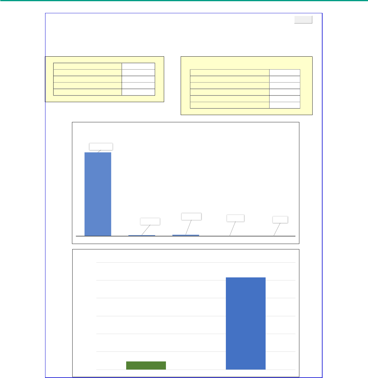
HIGHWAY SAFETY BENEFIT COST ANALYSIS GUIDE CHAPTER 8

131

Figure 25. Chart. Tabular and graphical BCA results from Highway Safety BCA

Tool.

AGENCY:

DOT

DATE

2/14/2018

Present

Present Value Costs ($ Dollars)

$900,000

ITEMIZED BENEFITS ($ Dollars) Value

Present Value Benefits ($ Dollars)

$10,318,036 $9,989,932

Net Present Value ($ Dollars) $9,418,036 $127,027

Benefit / Cost Ratio: 11.46 $182,431

Discount Rate 3.0% $16,749

$1,896

TOTAL BENEFITS $10,318,036

Emissions

Case 1, Alternative 2

Benefit-Cost Analysis Summary Results

Safety

Travel Time

Reliability

Vehicle Operating Cost

$9,989,932

$127,027

$182,431

$16,749

$1,896

SAFETY TRAVEL TIME RELIABILITY VEHICLE OPERATING COST EMISSIONS

Benefits Summary (Present Value, Dollars)

$900,000

$10,318,036

$2,000,000

$4,000,000

$6,000,000

$8,000,000

$10,000,000

$12,000,000

1 2

Benefits vs. Costs (Present Value, Dollars)

Costs

Benefits

HIGHWAY SAFETY BENEFIT COST ANALYSIS GUIDE CHAPTER 8

132

Figure 26 and Figure 27 present examples of tabular displays of BCA results from the FHWA

Tool for Operations Benefit-Cost Analysis (TOPS-BC) and the Clear Roads Cost-Benefit

Analysis Toolkit, respectively.

(37,38)

Similar to the Highway Safety BCA Tool, the TOPS-BC tool

presents the individual benefits for various categories such as travel time, travel time reliability,

energy, and safety; however, these costs and benefits represent annual values rather than net

present values. The Clear Roads tool includes a summary of the project parameters such as the

analysis period, discount rate, and itemized costs. The Clear Roads tool also separates agency

benefits, user (motorist) benefits, and society benefits.

Figure 26. Chart. Tabular BCA results from TOPS-BC tool.

(37)

Choose the active strategies: Benefit/Cost Summary

1 Link Based

Generic Link Analysis

Signal Coord.

Signal-Central

Signal Coordination: Central Control

Ramp Metering

RM-Preset

Ramp Metering: Preset Timing

3 Annual Benefits

1 TIM

TIM-FSP

Traffic Incident Management

4 Travel Time $

Dynamic Message Sign

ATIS-DMS

Dynamic Message Sign

Travel Time Reliability

Highway Advisory Radio

ATIS-HAR

Highway Advisory Radio

6 Energy $

Pre Trip Info

ATIS-511

Pre Trip Traveler Information

7 Safety $

1 HOT

ATDM-HOT

HOT Lanes

8 Other $

Hard Shoulder

ATDM-Shoulder

Hard Shoulder Running

9 User Entered $

1 Speed

ATDM-Speed

Speed Harmonization

10 Total Annual Benefits $

Weather Sys

Weather Mgmt

Road Weather Management

Work Zone

WorkZone

Work Zone Systems

12 Annual Costs $

Support-TMC

Traffic Management Center

Support-Loops

Loop Detection

14 Benefit/Cost Comparison

Support-CCTV

CCTV 15 Net Benefit $

Benefit Cost Ratio

Stream of Net Benefits

45,267

183,552

1.72

2.10

107,788

350,132

19,200

98,464

31,023

106,602

21,004

23,412

36,561

121,654

Generic Link

Analysis

Signal

Coordination:

Central Control

62,521

166,580

Generic Link Analysis

Signal Coordination: Central Control

Ramp Metering: Preset Timing

Traffic Incident Management

Dynamic Message Sign

Highway Advisory Radio

Pre Trip Traveler Information

HOT Lanes

Hard Shoulder Running

Speed Harmonization

Road Weather Management

Work Zone Systems

Traffic Management Center

Loop Detection

CCTV

HIGHWAY SAFETY BENEFIT COST ANALYSIS GUIDE CHAPTER 8

133

Figure 27. Chart. Tabular BCA results from Clear Roads cost-benefit tool.

(38)

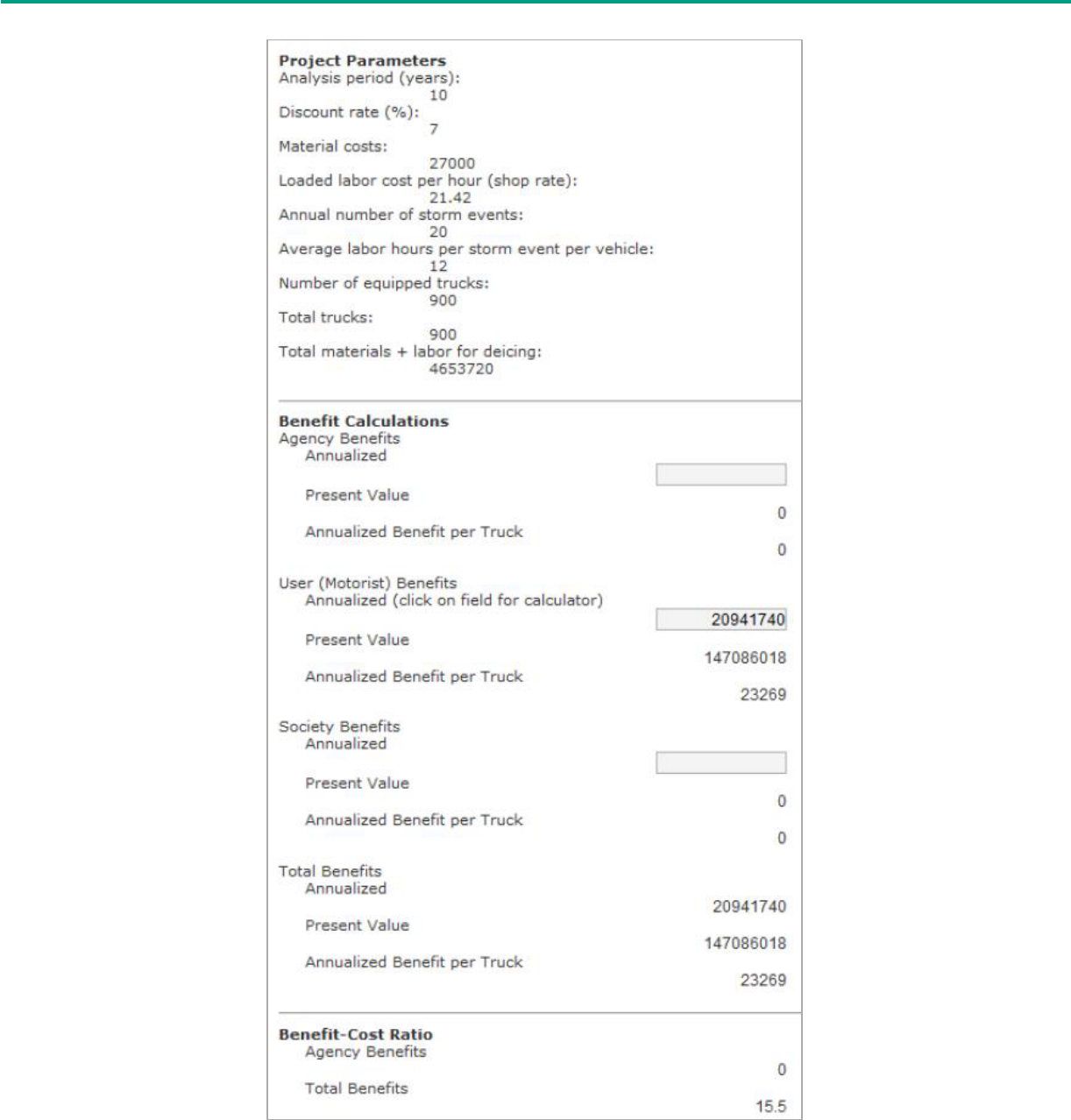
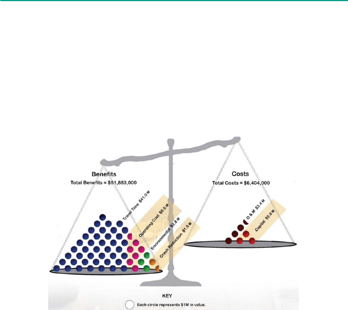
HIGHWAY SAFETY BENEFIT COST ANALYSIS GUIDE CHAPTER 8

134

This tabular output is often all that is needed by decision-makers; however, simple graphics can

enhance communication, providing a visually-informative display of results. Simple graphics can

aid in the understanding and interpretation of results, particularly for public officials and the

public. It may be difficult for a non-technical audience to comprehend and compare numbers in

a table, but a side-by-side graphical comparison, such as a bar chart, provides for much easier

comparison. Several such graphic displays are discussed and displayed below.

Simple graphics can enhance communication of BCA results.

Figure 28 is one example of a simple graphical display from a Kansas City SCOUT program

benefit-cost study. This graphic captures the essence of BCA, which is to provide a comparison

of the benefits received from an expenditure of costs. It also conveys the relative importance of

benefit and cost components to the overall benefit-cost ratio.

Figure 28. Chart. Graphical BCA results from Kansas City SCOUT.

(39)

As another example, the Southwestern Pennsylvania Regional Traffic Signal Program used a

“newsletter” approach to highlight the BCA results for a completed project. Figure 29 shows

the format of this BCA display technique, which includes detailed information about the

project., graphical displays of the first year of user benefits (number of stops and travel time),

the dollar value of total benefits, and the BCR.

HIGHWAY SAFETY BENEFIT COST ANALYSIS GUIDE CHAPTER 8

135

Figure 29. Chart. Newsletter display of BCA results from Southwestern Pennsylvania Regional Signal Program.

(9)

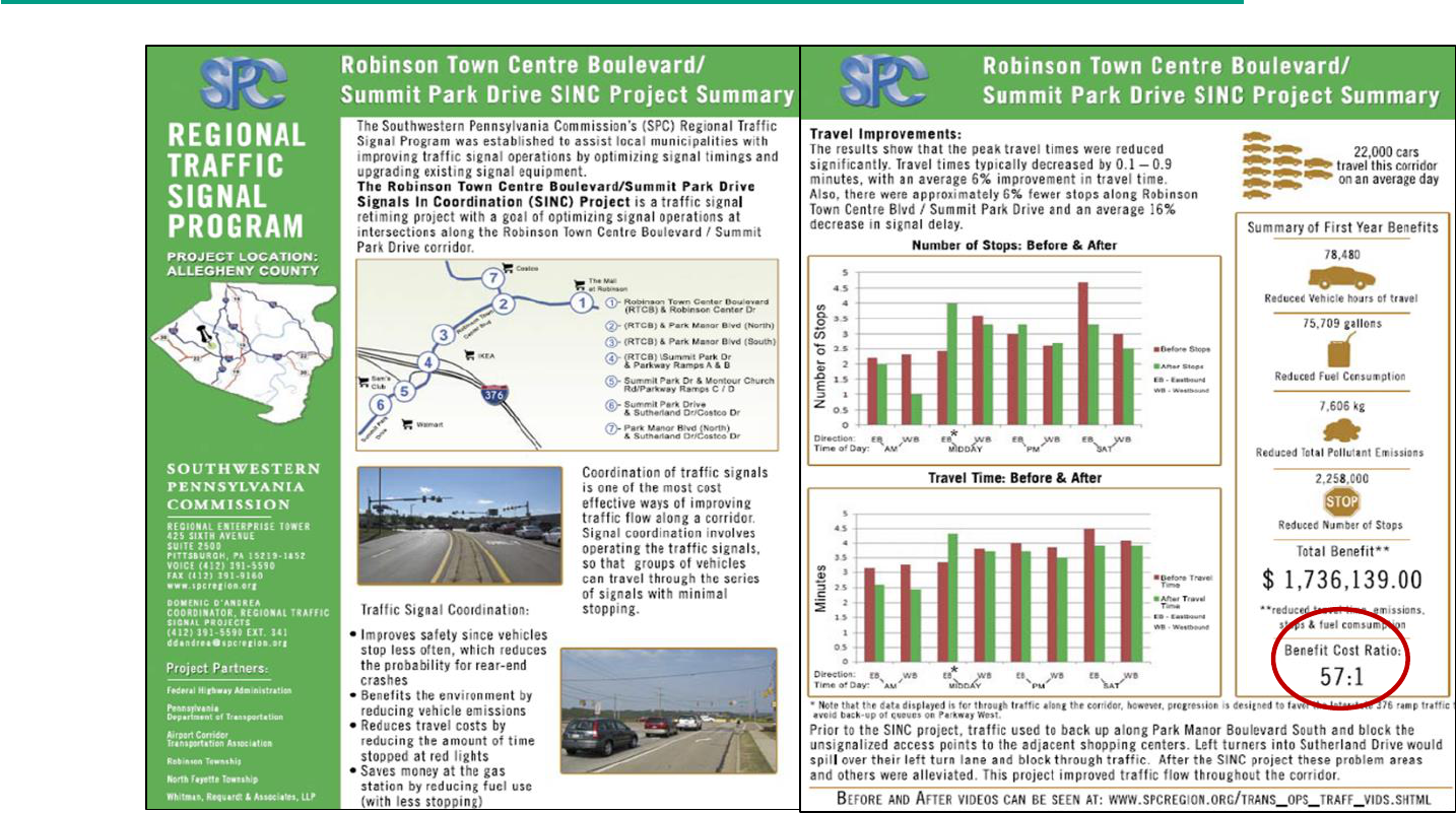
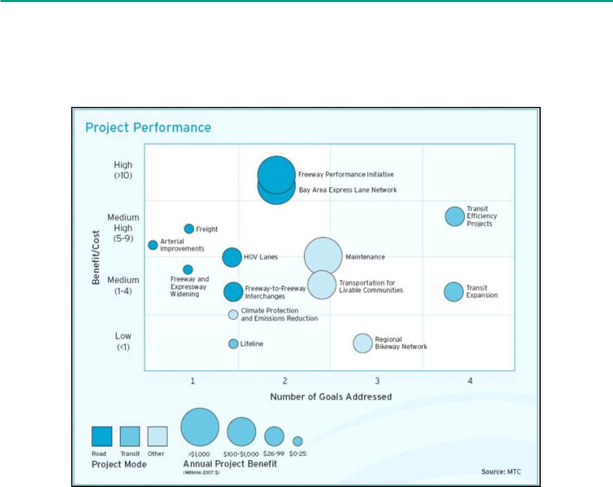
HIGHWAY SAFETY BENEFIT COST ANALYSIS GUIDE CHAPTER 8

136

Finally, graphical displays can seek to present a large amount of information in a single display.

The Metropolitan Transportation Commission (MTC) in the San Francisco Bay Area provided

multimodal BCA evaluation results, displaying the magnitude of the BCA results for each of the

various project performance measures concurrently (see Figure 30).

Figure 30. Chart. Multidimensional graphical BCA results from the Metropolitan

Transportation Commission.

(9)

In addition to communicating the BCA results to decision-makers, analysts can use tabular and

graphical summaries as part of a sensitivity analysis. These displays can help the analyst to

quickly compare the results among selected project assumptions. For example, Table 77

presents the results for the same alternative with two different assumptions for discount rate.

The results are notably different under the two assumptions.

HIGHWAY SAFETY BENEFIT COST ANALYSIS GUIDE CHAPTER 8

137

Analysts can use tabular and graphical

summaries to support sensitivity analysis.

Table 77. BCA results for multiple sites example.

Benefit Category

3% Discount Rate

7% Discount Rate

Crash Benefits

$10,690,130

$7,327,701

Travel Time Benefits

$28,933

$19,832

Vehicle Operating Cost Benefits

$1,858

$1,274

Emissions Benefits

$239

$164

Travel Time Reliability Benefits

$33,098

$23,668

Present Value Benefits ($ Dollars)

$10,754,258

$7,372,639

Present Value Costs ($ Dollars)

$620,356

$508,859

Net Present Value ($ Dollars)

$10,133,902

$6,863,780

Benefit-Cost Ratio

17.34

14.49

8.3 CHAPTER SUMMARY

Chapter 8 presents several considerations and options for communicating BCA results to

decision-makers and other potential audiences. The chapter begins with a discussion of several

considerations for communicating results. It then presents several examples, illustrating tabular

and graphical formats as well as different types of information that may be of interest in a

summary report.

Key Takeaways from Chapter 8:

• The effort to conduct a BCA is unproductive unless decision-makers use the results to

inform decisions.

• Balance tabular information with graphical displays.

• Simple graphics can enhance communication of BCA results.

• Analysts can use tabular and graphical summaries to support sensitivity analysis.

HIGHWAY SAFETY BENEFIT COST ANALYSIS GUIDE CHAPTER 8

138

THIS PAGE IS INTENTIONALLY LEFT BLANK

HIGHWAY SAFETY BENEFIT COST ANALYSIS GUIDE CHAPTER 9

139

9. SUMMARY

The purpose of this Guide is to assist transportation agencies in evaluating the economic

effectiveness and efficiency of projects and programs in support of consistent and sound

decision-making. This Guide introduces the BCA process and describes fundamental concepts

and factors to consider when preparing for BCA. It also describes some of the more complex

analytical concepts and the latest research to support more advanced BCA. Some of the more

advanced topics covered in this Guide include quantifying the long-term safety performance of

alternatives, estimating the safety impacts of multiple countermeasures, and capturing the

derivative safety benefits such as changes in travel time, reliability, delay, and air emissions that

result from fewer crashes.

The following are specific benefits to employing BCA in the roadway safety management and

project development processes:

• Documentation of Decision Process: The discipline of quantifying and valuing the

benefits and costs of highway projects also provides documentation to justify and

explain the decision process to legislatures and the public.

• Cost-Effective Design and Construction: Economic analysis can inform agencies as

to which of several project designs to implement at the lowest lifecycle cost to the

agency, lowest work zone delay cost to the traveler, highest safety benefit to highway

users, and the best affordable balance between these costs.

• Best Return on Investment: Economic analysis can help in planning, programming,

and implementing transportation programs with the best rate of return for any given

budget. It can also help to determine an optimal program budget.

• Understanding Complex Projects: In a time of growing public scrutiny of new and

costly road projects, transportation agencies and other decision makers need to

understand the comprehensive costs and benefits of these projects. A rigorous BCA can

help to quantify and compare the impacts of project alternatives on safety, mobility, the

environment, and regional economies.

A BCA attempts to capture all benefits to society from a project or course of action, and the

cost to achieve those benefits, regardless of which party realizes the benefits and costs, or the

form of these benefits and costs. A BCA should include project costs, user benefits, and non-

user benefits (externalities) to identify the preferred alternative. Ideally, the level of effort that

analysts allocate to quantifying benefits and costs in the BCA should be commensurate to the

expense, complexity, and controversy of the project. Transportation professionals can use BCA

to compare present value costs and benefits among alternatives. Used properly, BCA reveals

the most economically-efficient investment alternative (i.e., the one that maximizes the net

benefits to society relative to the allocation of resources).

HIGHWAY SAFETY BENEFIT COST ANALYSIS GUIDE CHAPTER 9

140

A BCA differentiates costs and benefits by project costs (or agency costs), project benefits (or

user benefits), and externalities (or non-user benefits). Project benefits and externalities include

costs avoided, but also include negative benefits (disbenefits) such as increased crashes or air

emissions. Analysts monetize project benefits by assigning dollar values to the different effects.

Project costs should include an accounting of all public-sector and private-sector costs, when

applicable. These costs represent:

• Initial capital costs of implementing the project, including planning, design,

construction/installation, and equipment costs.

• Continuing operations and maintenance costs necessary to keep the project operational,

including items such as power, communications, labor, and routine maintenance

(excludes replacement costs).

• Replacement cost of equipment that reaches the end of its useful life during the time

horizon of the analysis.

• “End of Project” costs necessary to close temporary projects or any residual or salvage

value of equipment at the end of the time horizon of the analysis.

Project benefits include reductions in crash frequency and severity, travel time and delay, and

vehicle operating costs. Externalities (or non-user benefits) include reductions in air emissions,

noise, and impacts to natural habitat and wetlands. These benefits and externalities may be a

direct benefit from the project or a residual benefit from a reduction in crashes.

Measuring the benefits of a safety project first requires estimates for the measures in the base

condition (e.g., the do-nothing alternative). The BCA estimates project benefits by calculating

changes between the base condition and project alternative(s). Where possible, the analyst

should estimate the safety benefits based on predicted or expected crash frequency rather than

observed crash frequency. A BCA uses the following measures to quantify project benefits and

disbenefits:

• Safety (frequency and severity of crashes).

• Mobility (travel time).

• Reliability (total delay).

• Vehicle operating cost (fuel and nonfuel use costs).

• Environment (emissions).

In BCA, the transportation professional applies a discount rate to the future annual benefits and

costs. The discount rate is the rate at which predicted cash expenditures (costs) or inflows

(benefits) decline in future years to reflect the time value of money. Once the analyst has

converted all benefits and costs to present values, there are several measures analysts can use

to compare alternatives in a BCA:

HIGHWAY SAFETY BENEFIT COST ANALYSIS GUIDE CHAPTER 9

141

• Benefit-cost ratio (BCR): The BCR is the ratio of present value benefits (including

negative benefits) to present value costs (initial and continuing costs over the project

lifecycle). In this context, the BCR is the same as the rate of return and return on

investment. A BCR greater than 1.0 indicates that benefits exceed costs, and the project

is economically justified. In general, a higher BCR is desirable. The BCR is most

appropriate for prioritizing project alternatives when funding restrictions apply (e.g.,

prioritizing locations or alternatives within a project with a fixed budget).

• Net present value (NPV): The NPV is the difference between present value benefits

and present value costs. NPV is also referred to as net benefits or net present worth. If

the NPV is greater than 0.0, then the benefits exceed the costs, and the project is

economically justified. In general, a higher NPV is desirable. An agency can use NPV to

determine the alternative with the highest net benefits for a given project.

• Cost-effectiveness index (CEI): The CEI is the average cost of a project to reduce

one crash. The CEI is calculated by dividing the present value cost (PVC) by the

expected crashes reduced over the service life of the project. In general, a low CEI is

desirable. The CEI is typically based on total crashes, but can be expressed in terms of a

specific crash type or severity level (e.g., cost to reduce one fatal and serious injury

crash). The CEI does not account for the magnitude of monetary benefits. As such, it is

not an appropriate measure to justify projects economically. It can, however, serve as a

measure when it is difficult to monetize benefits (e.g., the cost per new transit rider).

USDOT recommends analysts use the NPV or BCR for most economic evaluations. Both

measures used in combination, as well as standalone present value costs and benefits, will

provide better information to agencies. If benefits exceed costs, the NPV is positive and the

BCR is greater than 1.0, indicating the project is potentially economically justifiable. Where two

or more alternatives for a project exist, the one with the highest NPV over an equivalent

analysis period provides the most net benefits. Within a budget, maximizing BCR among

countermeasures or locations within a project provides the greatest economic efficiency. Policy

considerations, perceived risk, funding availability, and other influences may also affect the

selection of an alternative. Analysts may use other available BCA measures depending on the

technical problem or the agency policy or preference.

In summary, BCA is critical to understanding the potential return on investment from potential

projects. Highway safety BCA allows State and local agencies to quantify and assess safety

impacts alongside other decision factors such as operational efficiency, environmental impacts,

and pavement preservation. While BCA is a policy or procedure decision, this Guide and

related spreadsheet tool will assist agencies in justifying the need to perform BCA, identifying

appropriate inputs and parameters for analysis, and conducting sound highway safety BCA to

evaluate the economic effectiveness and efficiency of projects. A reliable BCA will help to

inform decisions and improve investments.

HIGHWAY SAFETY BENEFIT COST ANALYSIS GUIDE CHAPTER 9

142

THIS PAGE IS INTENTIONALLY LEFT BLANK

HIGHWAY SAFETY BENEFIT COST ANALYSIS GUIDE REFERENCES

143

REFERENCES

1. Sallman, D., E. Flanigan, K. Jeannotte, C. Hedden, and D. Morallos, Operations Benefit/Cost

Analysis Desk Reference, FHWA-HOP-12-028, Federal Highway Administration,

Washington, DC, 2012. Accessed February 2018 at:

http://ops.fhwa.dot.gov/publications/fhwahop12028/fhwahop12028.pdf.

2. Srinivasan, R., F. Gross, B. Lan, and G. Bahar. Reliability of Safety Management Methods:

Network Screening, FHWA-SA-16-037, Federal Highway Administration, Washington,

DC, 2016.

3. Srinivasan, R., G. Bahar, and F. Gross. Reliability of Safety Management Methods: Diagnosis,

Report No. FHWA-SA-16-038, Federal Highway Administration, Washington, D.C.,

November 2016.

4. Bahar, G., R. Srinivasan, and F. Gross. Reliability of Safety Management Methods:

Countermeasure Selection, Report No. FHWA-SA-16-039, Federal Highway

Administration, Washington, D.C., August 2016.

5. Code of Federal Regulations, Highway Safety Improvement Program, 23 CFR 924.3,

Accessed February 2018 at:

https://www.fhwa.dot.gov/legsregs/directives/fapg/cfr0924.htm.

6. Gross, F., T. Harmon, G. Bahar, and K. Peach. Reliability of Safety Management Methods:

Systemic Safety Programs, FHWA-SA-16-041, Federal Highway Administration,

Washington, DC, 2016.

7. American Association of State Highway and Transportation Officials (AASHTO),

Highway Safety Manual, 1

Edition, 2010.

8. US Department of Transportation, Economic Analysis Primer, FHWA-IF-03-032, Federal

Highway Administration, Washington, DC, 2003. Accessed February 2018 at:

http://www.webpages.uidaho.edu/~mlowry/Teaching/EngineeringEconomy/Supplemental/

USDOT_Economic_Analysis_Primer.pdf.

9. Lawrence, M., P. Nguyen, J. Skolnick, J. Symoun, J. Hunt, and R. Alfelor. Transportation

Systems Management and Operations Benefit-Cost Analysis Compendium, FHWA-HOP-14-

032, Federal Highway Administration, Washington, DC, 2015. Accessed February 2018

at: https://ops.fhwa.dot.gov/publications/fhwahop14032/index.htm.

10. Harmon, T., G. Bahar, and F. Gross. Crash Costs for Highway Safety Analysis, FHWA-SA-

17-071, Federal Highway Administration, Washington, DC, 2018. Accessed February

2018 at: https://safety.fhwa.dot.gov/hsip/planning.cfm.

HIGHWAY SAFETY BENEFIT COST ANALYSIS GUIDE REFERENCES

144

11. Blincoe, L.J., T.R. Miller, E. Zaloshnja, and B.A. Lawrence. The Economic and Societal

Impact Of Motor Vehicle Crashes, 2010 (Revised), DOT-HS-812-013, National Highway

Traffic Safety Administration, Washington, DC, 2015. Accessed February 2018 at:

https://crashstats.nhtsa.dot.gov/Api/Public/ViewPublication/812013.

12. US Department of Transportation, Life-Cycle Cost Analysis Primer, Federal Highway

Administration, Washington, DC, 2002. Accessed February 2018 at:

https://www.fhwa.dot.gov/asset/lcca/010621.pdf.

13. US Department of Transportation, Benefit-Cost Analysis Guidance for TIGER and INFRA

Applications, Office of the Secretary, Washington, DC, 2017. Accessed February 2018 at:

https://www.transportation.gov/office-policy/transportation-policy/benefit-cost-analysis-

guidance.

14. Herbel, S., L. Laing, and C. McGovern, Highway Safety Improvement Program Manual,

FHWA-SA-09-029, Federal Highway Administration, Washington, DC, 2010. Accessed

February 2018 at:

http://safety.fhwa.dot.gov/hsip/resources/fhwasa09029/fhwasa09029.pdf.

15. CMF Clearinghouse. Federal Highway Administration, Washington, DC. Accessed

February 2018 at: http://www.cmfclearinghouse.org.

16. Transportation Research Board. Determining Highway Maintenance Costs, Report 688,

National Cooperative Highway Research Program, Washington, DC, 2011. Accessed

February 2018 at: http://www.trb.org/Publications/Blurbs/165504.aspx.

17. Smith, S. and K. Signor. Synthesis of Countermeasure Cost User Guide, FHWA-SA-16-012,

Federal Highway Administration, Washington, DC, 2017. Accessed February 2018 at:

http://www.cmfclearinghouse.org/resources_synthesisofcountermeasurecosts.cfm.

18. US Department of Transportation, Service Life and Crash Cost User Guide, Federal

Highway Administration, Washington, DC, 2017. Accessed February 2018 at:

http://www.cmfclearinghouse.org/resources_servlifecrashcostguide.cfm.

19. Adams, T.M. Estimating Cost Per Lane Mile for Routine Highway Operations and

Maintenance, MRUTC 07-12, Wisconsin Department of Transportation, Madison, WI,

2011. Accessed February 2018 at: http://www.wistrans.org/mrutc/files/CPLM_Final.pdf.

20. US Department of Transportation. MMUCC Guideline—Model Minimum Uniform

Crash Criteria 5

Edition, DOT-HS-812-433, National Highway Traffic Safety

Administration, July 2017. Accessed February 2018 at:

https://crashstats.nhtsa.dot.gov/Api/Public/Publication/812433.

HIGHWAY SAFETY BENEFIT COST ANALYSIS GUIDE REFERENCES

145

21. Association for the Advancement of Automotive Medicine. Abbreviated Injury Scale, 2015.

Accessed February 2018 at: https://www.aaam.org/abbreviated-injury-scale-ais/.

22. Hagemann, G., K. Hymel, A. Klauber, D.B. Lee, G. Noel, D. Pace, and C. Taylor. Delay

and Environmental Costs of Truck Crashes. FMCSA-RRA-13-043, Federal Motor Carrier

Safety Administration, Washington, DC, 2013. Accessed February 2018 at:

https://rosap.ntl.bts.gov/view/dot/10074.

23. US Department of Transportation, Tiger Benefit-Cost Analysis (BCA) Resource Guide,

3/27/15, Accessed February 2018 at:

https://www.transportation.gov/sites/dot.gov/files/docs/Tiger_Benefit-

Cost_Analysis_%28BCA%29_Resource_Guide_1.pdf.

24. Memorandum to Secretarial Officers and Modal Administrators, “Revised Departmental

Guidance on Valuation of Travel Time in Economic Analysis” from Polly Trottenberg,

Assistant Secretary for Transportation Policy, Prepared by Peter Belenky, Economist,

September 29, 2011.

25. Victoria Transport Policy Institute, Transportation Cost and Benefit Analysis II – Travel Time

Costs, January 2017, Accessed February 2018 at: http://www.vtpi.org/tca/tca0502.pdf.

26. Mallett, W., C. Jones, J. Sedor, and J. Short. Freight Performance Measurement: Travel Time

in Freight-Significant Corridors, FHWA-HOP-07-071, Federal Highway Administration,

Washington, DC, 2006. Accessed February 2018 at:

http://ops.fhwa.dot.gov/freight/freight_analysis/perform_meas/fpmtraveltime/traveltimebr

ochure.pdf.

27. Transportation Research Board. Analytical Procedures for Determining the Impacts of

Reliability Mitigation Strategies, S2-L03-RR-1, Second Strategic Highway Research Program,

Washington, DC, 2013, Accessed February 2018 at:

http://www.trb.org/Publications/Blurbs/166935.aspx.

28. US Department of Transportation. Travel Time Reliability: Making it There on Time, All the

Time, FHWA-HOP-06-070, Federal Highway Administration, Washington, DC, 2006,

Accessed February 2018 at:

https://ops.fhwa.dot.gov/publications/tt_reliability/TTR_Report.htm.

29. US Energy Information Administration. Annual Energy Outlook, 2017 with projections to

2050, Washington, DC, January 5, 2017. Accessed February 2018 at: www.eia.gov/aeo.

30. US Energy Information Administration. Gasoline and Diesel Fuel Update, Washington, DC.

Accessed February 2017 at: https://www.eia.gov/petroleum/gasdiesel/.

HIGHWAY SAFETY BENEFIT COST ANALYSIS GUIDE REFERENCES

146

31. American Automobile Association, Your Driving Costs – 2016 Edition (2016), AAA

Association Communication, Heathrow, FL, 2016. Accessed February 2018 at:

http://exchange.aaa.com/automotive/driving-costs/#.WVZdF02oupp.

32. Torrey, W.F. and D. Murray. An Analysis of the Operational Costs of Trucking: 2016 Update

(2016), American Transportation Research Institute, Arlington, Virginia, September

2016. Accessed February 2018 at: http://atri-online.org/wp-

content/uploads/2016/10/ATRI-Operational-Costs-of-Trucking-2016-09-2016.pdf.

33. US Department of Labor. Archived Consumer Price Index Detailed Reports. Bureau of Labor

Statistics, August 2017. Accessed February 2018 at: https://www.bls.gov/cpi/detailed-

report.htm.

34. US Department of Transportation, Crash Modification Factors in Practice—Quantifying

Safety in the Roadway Safety Management Process, FHWA-SA-13-010, Federal Highway

Administration, Washington, DC, 2013. Accessed February 2018 at:

https://safety.fhwa.dot.gov/tools/crf/resources/cmfs/management.cfm.

35. Carter, D., R. Srinivasan, B. Persaud, C. Lyon, F. Gross, S. Himes, T. Le, J. Bonneson, and

E. Hauer. Guidance for the Development and Application of Crash Modification Factors. Final

Report, Project 17-63, National Cooperative Highway Research Program, Washington,

DC, March 2017.

36. Transportation Research Board, Development of Tools for Assessing Wider Economic

Benefits of Transportation, S2-C11-RW-1, Second Strategic Highway Research Program,

Washington, DC, 2014. Accessed February 2018 at:

http://www.trb.org/Publications/Blurbs/169524.aspx.

37. US Department of Transportation, Tool for Operations Benefit-Cost Analysis, Federal

Highway Administration, Washington, DC. Accessed February 2018 at:

https://ops.fhwa.dot.gov/plan4ops/topsbctool/index.htm.

38. Clear Roads Cost-Benefit Analysis Toolkit: Accessed February 2018 at:

http://clearroads.org/cba-toolkit/terms.html.

39. Kansas and Missouri Departments of Transportation, Kansas City Scout Annual Report,

2015. Accessed February 2018 at:

http://www.kcscout.net/downloads/Reports/Annual/AnnualReport2015.pdf.

HIGHWAY SAFETY BENEFIT COST ANALYSIS GUIDE APPENDIX A

147

APPENDIX A: GLOSSARY OF TERMS

TERM

DEFINITION

Benefit-Cost Analysis

A systematic process for calculating and comparing benefits

and costs of a project.

Benefit/Cost Ratio

Measure calculated by dividing the incremental monetized

benefits related to a project by the incremental costs of that

project. May either be expressed as a ratio (2:1) or a

resultant value (2). B/C ratios greater than one indicate that

a project is efficient (benefits exceed costs). B/C ratios less

than one indicate that a project is inefficient (costs exceed

benefits).

Countermeasure

Roadway-based strategy intended to reduce the crash

frequency or severity, or both at a site.

Crash Modification Factor

Multiplicative factor used to compute the expected number

of crashes after implementing a given countermeasure.

Crash Reduction Factor

The percentage crash reduction that might be expected after

implementing a given countermeasure.

Direct Benefits

Those measurable benefits that may be directly attributed to

the project investment.

Discount Rate

The rate at which predicted cash expenditures (costs) or

inflows (benefits) are reduced in future years to reflect the

time cost of money. The purpose of the discount rate is to

convert future values to present value.

Efficient

Projects determined to have benefits greater than their costs

and are economically justifiable (B/C ratio greater than one).

Externality

The uncompensated impact of one person's actions on the

well-being of a bystander. In the case of transportation

investments, "bystanders" are the nonusers of the project.

When the impact benefits the nonuser, this is called a

positive externality. When the impact is adverse, this is

called a negative externality.

Inefficient

Projects determined to have benefits less than their costs

and are economically unjustifiable (B/C ratio less than one).

Life-Cycle Costs

All costs accruing to highway agencies and to users of the

highway system as a result of agency construction and

maintenance activities. These costs include initial

construction, maintenance, rehabilitation and end-of-life

HIGHWAY SAFETY BENEFIT COST ANALYSIS GUIDE APPENDIX A

148

TERM

DEFINITION

costs, as well as user costs such as vehicle operating, travel

time and crash costs associated with work zones.

Measure of Effectiveness

Metric used to evaluate the level of impact of a project.

Net Benefit

The sum of a project benefits minus the sum of the project

costs.

Net Present Value

The sum of the discounted stream of expected benefits and

costs over a selected time horizon.

Operations and Maintenance

Costs

The continuing costs necessary to keep the project

performing as planned, including items, such as power,

communications, labor, and routine maintenance.

Replacement Costs

The cost of replacing equipment that reaches the end of its

useful life during the time horizon of the analysis.

Safety Performance Function

An equation used to predict the average number of crashes

per year at a location as a function of exposure and, in some

cases, roadway or intersection characteristics.

Time Cost of Money

The impact of time on the value of future benefits and costs.

Money spent or earned today is more valuable than the same

amount of money promised in a future year since the money

earned today can be invested and earn additional revenue in

the interim years. Therefore, benefits and costs accruing in

later years of an analysis are often valued at a discounted

rate.

Value of a Statistical Life

Additional cost that individuals would be willing to bear for

improvements in safety (that is, reductions in risks) that, in

the aggregate, reduce the expected number of fatalities by

one.

For More Information:

Visit https://safety.fhwa.dot.gov/

FHWA, Ofﬁce of Safety

Karen Scurry

[email protected]

609-637-4207

FHWA-SA-18-001